The benchmark problems are presented in the page BENCHMAX.

Authors, affiliation

Authors
Philipp FRAUENFELDER, Kersten SCHMIDT, Christoph SCHWAB.

Affiliation
ETH Zürich, Seminar for Applied Mathematics

Method and code

The method is the weighted Regularization.

It consists in adding to the bilinear form \int_Domain curl u . curl v dx a part in s \int_Domain div u div v d\mu with, instead the standard measure dx on the Domain, a measure of the form d\mu = \rho(x) dx where \rho(x) is a suitable weight (it tends to zero with a special rate as x tends to the singular support of the solution). s is a scaling parameter not affecting physical Eigenmodes.

Reference 1:
Martin COSTABEL, Monique DAUGE,
"Weighted Regularization of Maxwell Equations in Polyhedral Domains. A rehabilitation of nodal finite elements", Numer. Math., 93(2): 239-277, 2002.

Reference 2:
Philipp FRAUENFELDER, Christian LAGE,
"Concepts-An Object-Oriented Software Package for Partial Differential Equations", M2AN Math. Model. Numer. Anal. 36(5): 937-951, 2002.

Reference 3:
Philipp FRAUENFELDER,
"hp-Finite Element Methods for Anisotropically, Locally Refined Meshes in Three Dimensions", Doctoral Dissertation, in preparation. (To be found online.)

Reference 4:
Code Concepts

Reference 5:
Mark AINSWORTH and Joe COYLE,
"Hierarchic hp-edge element families for Maxwell's equations on hybrid quadrilateral/triangular meshes", Comput. Methods Appl. Mech. Engrg. 190(49-50): 6709-6733, 2001.

Reference 6:
Paul David LEDGER,
"An hp-adaptive finite element procedure for electromagnetic scattering problems", Doctoral Dissertation, University of Wales, Nov. 2001.

Technical data:
Computations in double precision arithmetics on a Sun-Fire-880 running Solaris 2.8. Eigensolver: ARPACK together with Umfpack as direct sparse linear solver.

Results

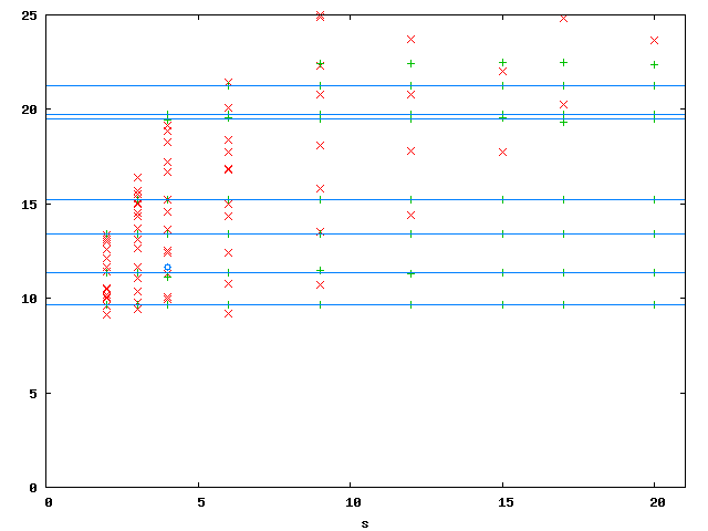
Maxwell eigenvalues in 2DomA (L-shape), (20031112)

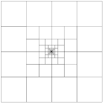
Computed by a Galerkin approximation with a geometric mesh with increasing number of layers n and linearly distributed polynomial degree (between 2 in the smallest two layers and n+1 in the largest layer).

Mesh

Eigenvalues

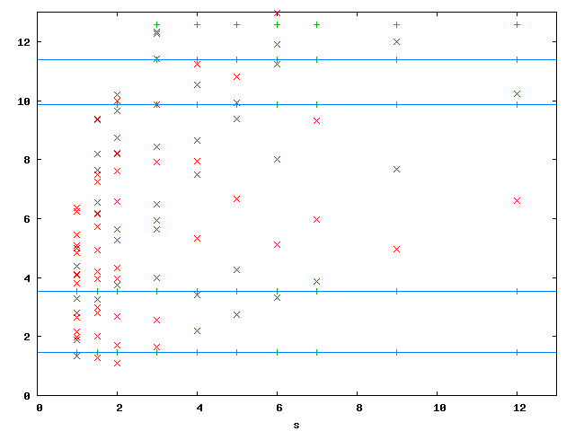
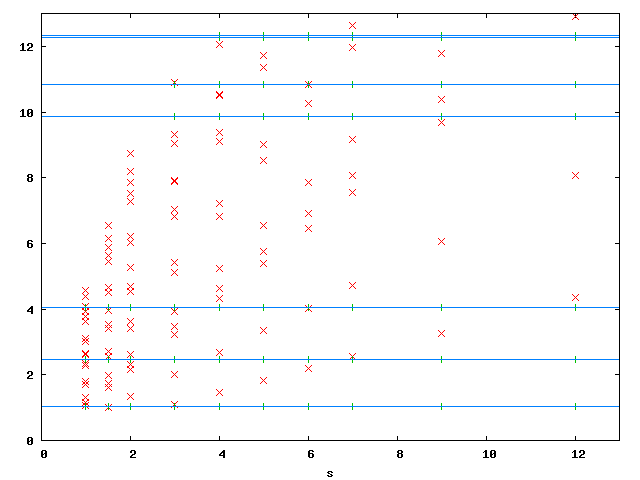
In the above plot (15770 dofs), red are spurious Eigenvalues, green are physical Eigenvalues, horizontal blue lines are 'exact' values from Benchmax. Below are the numeric values of the first three physical Eigenvalues for different number of layers n. We chose s = 9.

Relative errors with benchmark

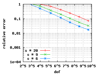
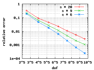
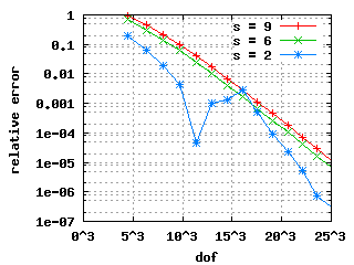
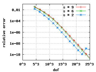
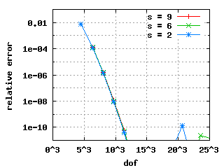
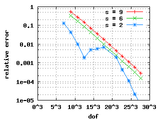
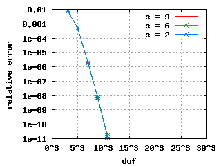
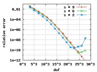
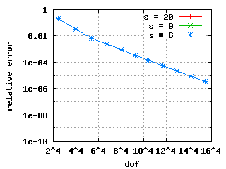
The convergence histories below for the 1st, 2nd and 3rd Eigenvalue show three different curves each: for the values s = 9, s = 6 and s = 2.

Maxwell eigenvalues in 2DomB (Cracked domain), (20031112)

Computed by a Galerkin approximation with a geometric mesh with increasing number of layers n and linearly distributed polynomial degree (between 2 in the smallest two layers and n+1 in the largest layer).

Mesh

We have meshed the whole domain despite of its symmetry.

Eigenvalues

In the above plot (21028 dofs), red are spurious Eigenvalues, green are physical Eigenvalues, horizontal blue lines are 'exact' values from Benchmax. Below are the numeric values of the first three physical Eigenvalues for different number of layers n. We chose s = 9.

Relative errors with benchmark

The convergence histories below for the 1st, 2nd and 3rd Eigenvalue show three different curves each: for the values s = 9, s = 6 and s = 2.

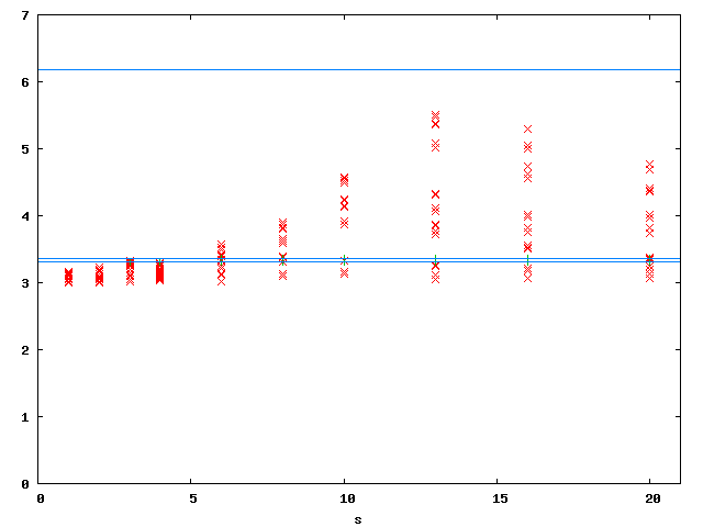
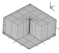
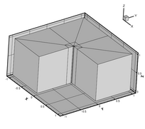
Maxwell eigenvalues in 2DomE (Square for transmission problems, ε₁ = 0.5), (20040408, 20040505, 20040511)

Computed by a Galerkin approximation with a geometric mesh with increasing number of layers n and linearly distributed polynomial degree (between 2 in the smallest two layers and n+1 in the largest layer). We have used three different methods:

• Plain weighted regularization: The domain is meshed in one piece. The mesh-degree combination is refined anisotropically towards the interfaces (see picture below) and the weight is chosen as w = min(|x|, |y|) (the interfaces coincide with the coordinate axis).
  We do not expect this method to give good results as an unbounded number of spurious modes appears in the discretization limit.
• Weighted regularization with node doubling at the interfaces and imposed constraints (tangential component continuous, normal component satisfying
  u_nl * eps_l + u_nr * eps_r = 0,
  ie. when eps_l = eps_r, continuity of the normal component is enforced. The weight is w = r, ie. the distance to the origin.
• Edge elements (see References 5 and 6).

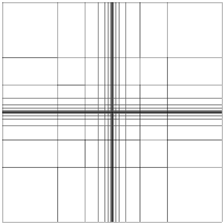
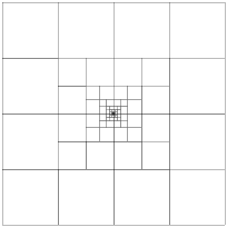
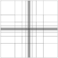
Plain Weighted Regularization	Weighted Regularization with Node Doubling	Edge Elements
Mesh
Eigenvalues
		N = 60 n = 1 N = 264 n = 2 3.31732589456964 3.35972173595939 6.18999459362659 3.31743364084025 3.36393612737339 6.18643980456594 N = 752 n = 3 N = 1692 n = 4 3.31752601416437 3.365511568792 6.18639017210705 3.31754451531046 3.36604952473317 6.18638955736896 N = 3284 n = 5 N = 5760 n = 6 3.31754797550072 3.36623145128975 6.1863895618935 3.31754861742566 3.36629287184557 6.1863895624481 N = 9384 n = 7 N = 14452 n = 8 3.31754873637201 3.36631360012794 6.18638956248473 3.31754875840574 3.36632059486052 6.18638956248701 N = 21292 n = 9 N = 30264 n = 10 3.31754876248696 3.36632295516737 6.18638956248675 3.31754876324292 3.36632375162601 6.18638956248728 N = 41760 n = 11 N = 56204 n = 12 3.3175487633826 3.36632402038143 6.18638956248719 3.31754876340893 3.36632411107011 6.18638956248657 N = 74052 n = 13 N = 95792 n = 14 3.31754876341618 3.36632414167234 6.18638956248975 3.31754876341594 3.36632415199731 6.18638956248872
In the above plots (20766 and 7680 dofs, click for larger version), red are spurious Eigenvalues, green are physical Eigenvalues, horizontal blue lines are 'exact' values from Benchmax. Below are the numeric values of the first three physical Eigenvalues for different number of layers n. We chose s = 10.
N = 30 n = 1 N = 126 n = 2 3.24322810224601 3.24577214731192 6.19564598036415 3.10046941236368 3.10880009755685 6.13597244613991 N = 382 n = 3 N = 918 n = 4 3.36429152443549 3.42602202134598 6.18615540859658 3.33088887534925 3.37976522991338 6.18672444106447 N = 1886 n = 5 N = 3470 n = 6 3.32412501143759 3.38087661290379 6.18643317284668 3.32157904777508 3.38885100742956 6.18633040958983 N = 5886 n = 7 N = 9382 n = 8 3.31814605198328 3.36045217405082 6.18763689455118 3.31801549367598 3.36774355773469   N = 14238 n = 9 N = 20766 n = 10 3.31774714738676 3.36708395225233   3.31763079225684 3.36664571697868	N = 48 n = 1 N = 160 n = 2 4.06896961214344 6.34172438800243 6.68558365532546 3.59983870638615 4.69979306038279 6.1955373161925 N = 400 n = 3 N = 792 n = 4 3.42710036046357 3.9098809313688 6.18672374063397 3.35682098891715 3.59501007357774 6.18643315752554 N = 1360 n = 5 N = 2128 n = 6 3.3301178668276 3.45892600252659 6.18639923312905 3.32096595687638 3.40120715628326 6.18639175159294 N = 3120 n = 7 N = 4360 n = 8 3.31832267907811 3.37877617228035 6.18639004454515 3.3177043505265 3.37063120234754 6.18638966502972 N = 5872 n = 9 N = 7680 n = 10 3.31757860067753 3.36779816676172 6.18638958395823 3.31755440928261 3.3668277420059 6.1863895669101
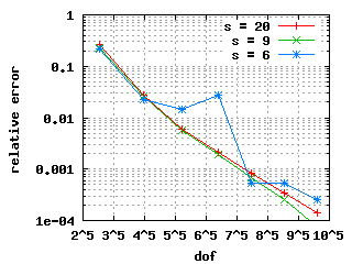
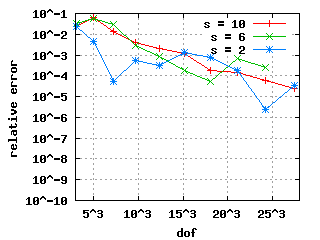
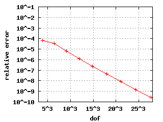
Relative errors with benchmark The convergence histories below for the 1st, 2nd and 3rd Eigenvalue show three different curves each: for the values s = 10, s = 6 and s = 2. In the case of edge elements, no s is used.
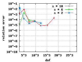
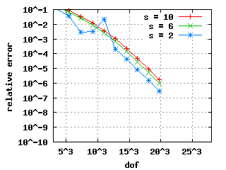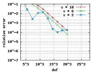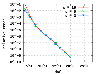
The descent for the weighted regularization with node doubling (pictures in the middle) is steeper because it uses only a vertex mesh as opposed to edge meshes in the other two cases.

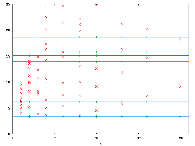
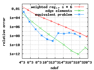
Maxwell eigenvalues in 2DomE (Square for transmission problems, ε₁ = 1e-2), (20040527)

Computed by a Galerkin approximation with a geometric mesh with increasing number of layers n and linearly distributed polynomial degree (between 2 in the smallest two layers and n+1 in the largest layer). We have used three different methods:

• Weighted regularization with node doubling at the interfaces and imposed constraints (tangential component continuous, normal component satisfying
  u_nl * eps_l + u_nr * eps_r = 0,
  ie. when eps_l = eps_r, continuity of the normal component is enforced. The weight is w = r, ie. the distance to the origin.
• Edge elements (see References 5 and 6).
• Equivalent magnetic problem (see Benchmax, scalar).

Mesh

The same mesh was used for all three methods.

Eigenvalues

In the above plot (7680 dofs), red are spurious Eigenvalues, green are physical Eigenvalues, horizontal blue lines are 'exact' values from Benchmax. Below are the numeric values of the first three physical Eigenvalues for different number of layers n. We chose s = 2.

Relative errors with benchmark

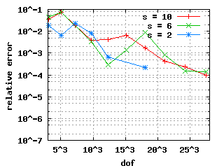
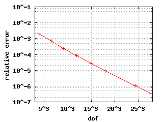
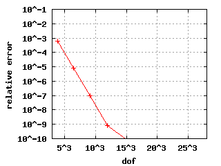
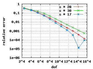
The convergence histories below for the 1st, 2nd and 3rd Eigenvalue

Remarks

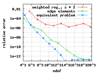
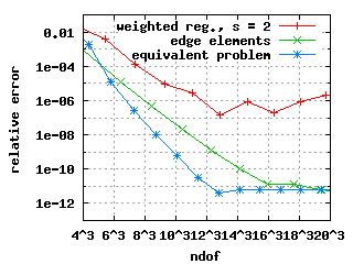
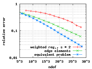
The edge elements and the equivalent problem show exponential convergence for the first three Eigenvalues in the above plots. The weighted regularisation only does so for the third Eigenvalue. The convergence histories for the first and second Eigenvalue deteriorate at a level of the relative error of 10^-6. This does not depend on s, the chosen Eigenvalue solver (or its parameters) or the formulation of the constraints at the origin.

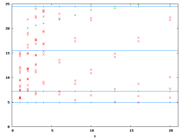
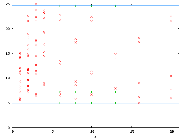
The third plot above shows the convergence history for the third Eigenvalue: It is approximated poorly. The reason is that the third Eigenfunction has a strong unbounded singularity at the origin. This can also be seen in the eigenvalues-s plot: The Eigenvalues computed with the weighted regularisation are above 20 for s >= 2 and even above 25 for s >= 16---the true value is expected to be close to 15.

Maxwell eigenvalues in 2DomE (Square for transmission problems, ε₁ = 1e-8), (20040512)

Computed by a Galerkin approximation with a geometric mesh with increasing number of layers n and linearly distributed polynomial degree (between 2 in the smallest two layers and n+1 in the largest layer). We have used three different methods:

• weighted regularization with node doubling at the interfaces and imposed constraints (tangential component continuous, normal component satisfying
  u_nl * eps_l + u_nr * eps_r = 0,
  ie. when eps_l = eps_r, continuity of the normal component is enforced.
• edge elements (see References 5 and 6)
• equivalent magnetic problem (see Benchmax)

Mesh

The same mesh was used for all three methods.

Eigenvalues

In the above plot (7680 dofs), red are spurious Eigenvalues, green are physical Eigenvalues, horizontal blue lines are 'exact' values from Benchmax. Below are the numeric values of the first three physical Eigenvalues for different number of layers n. We chose s = 6.

Relative errors with benchmark

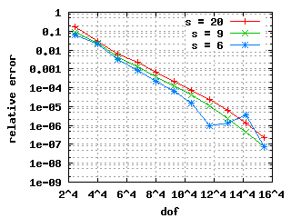
The convergence histories below for the 1st, 2nd and 3rd Eigenvalue

Remarks

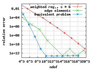
All three methods show exponential convergence for the first three Eigenvalues in the above plots with the following two exceptions:

• The equivalent magnetic problem is only able to resolve the second Eigenvalue up to a relative precision of 10^-7. This has been confirmed for different meshes, refinements and parameters for the Eigensolver.
• The third Eigenvalue can only be resolved up to a relative precision of 10^-7 The reason is that the third and fourth Eigenvalue are very close:
  (λ₄ - λ₃)/λ₄ = 10^-7,
  this results in an ill-conditioned matrix Eigenproblem. The Eigensolver ARPACK has problems yielding high accuracy under these circumstances.

Maxwell eigenvalues in 3DomA (thick L), (20031124)

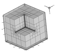
Computed by a Galerkin approximation with a geometric mesh with increasing number of layers n and linearly distributed polynomial degree (between 1 in the smallest two layers and n in the largest layer). We used two different geometric grading parameters: σ = 0.5 and σ = 0.15.

Mesh

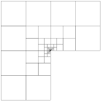
The mesh with σ = 0.5 on the left has hanging nodes and is automatically generated by refining geometrically towards the singular reentrant edge. The mesh with σ = 0.15 on the right is generated by and hand-written mesh generator and is regular (no hanging nodes).

Eigenvalues for σ = 0.5

In the above plot (18726 dofs), red are spurious Eigenvalues, green are physical Eigenvalues, blue circles are undecided, horizontal blue lines are 'exact' values from Benchmax. Below are the numeric values of the first three physical Eigenvalues for different number of layers n. We chose s = 9.

Eigenvalues for σ = 0.15

Relative errors with benchmark for σ = 0.5 and σ = 0.15

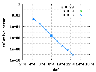
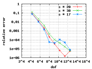
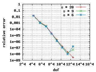
The convergence histories below for the 1st, 2nd and 3rd Eigenvalue (top to bottom) show three different curves each for different values of s. The left and right plots show σ = 0.5 and σ = 0.15 respectively with the same scales! It is clearly visible that the mesh with σ = 0.15 beats the mesh with σ = 0.5. Note: the convergence histories for the different values of s are identical for the 1st Eigenvalue.

σ = 0.5	σ = 0.15

Maxwell eigenvalues in 3DomB (Fichera), (20031127)

Computed by a Galerkin approximation with a geometric mesh with increasing number of layers n and linearly distributed polynomial degree (between 1 in the smallest two layers and n in the largest layer).

Mesh

Eigenvalues

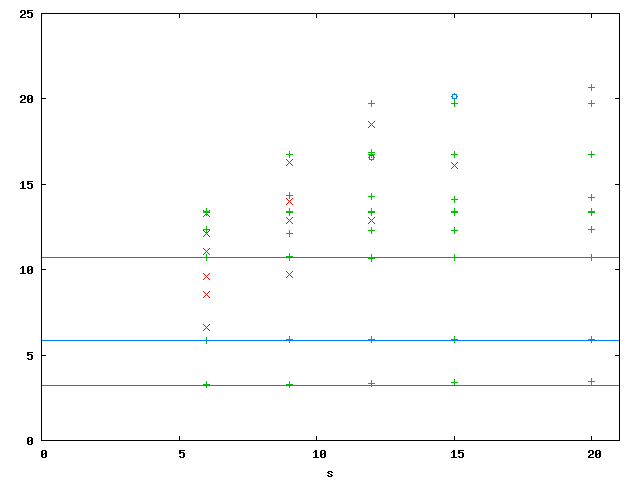
In the above plot (45450 dofs), red are spurious Eigenvalues, green are physical Eigenvalues, blue circles are undecided, horizontal blue lines are extrapolated values from the computations.

Below are the numeric values of the first three physical Eigenvalues for different number of layers n. We chose s = 9.

Relative errors with benchmark

The convergence histories below for the 1st, 2nd and 3rd Eigenvalue show three different curves each: for the values s = 9, s = 6 and s = 2.