Web page of Florian Feppon

This page provides a brief outline of the null space algorithm for nonlinear constrained optimization developped in full details in

Abstract: The purpose of this article is to introduce a gradient-flow algorithm for solving generic equality or inequality constrained optimization problems, which is suited for shape optimization applications. We rely on a variant of the Ordinary Differential Equation (ODE) approach proposed by Yamashita for equality constrained problems: the search direction is a combination of a null space step and a range space step, which are aimed to reduce the value of the minimized objective function and the violation of the constraints, respectively. Our first contribution is to propose an extension of this ODE approach to optimization problems featuring both equality and inequality constraints. In the literature, a common practice consists in reducing inequality constraints to equality constraints by the introduction of additional slack variables. Here, we rather solve their local combinatorial character by computing the projection of the gradient of the objective function onto the cone of feasible directions. This is achieved by solving a dual quadratic programming subproblem whose size equals the number of active or violated constraints, and which allows to identify the inequality constraints which should remain tangent to the optimization trajectory. Our second contribution is a formulation of our gradient flow in the context of-infinite-dimensional-Hilbert space settings. This allows to extend the method to quite general optimization sets equipped with a suitable manifold structure, and notably to sets of shapes as it occurs in shape optimization with the framework of Hadamard's boundary variation method. The cornerstone of this latter setting is the classical operation of extension and regularization of shape derivatives. Some numerical comparisons on simple academic examples are performed to illustrate the behavior of our algorithm. Its numerical efficiency and ease of implementation are finally demonstrated on more realistic shape optimization problems.

@article{feppon2020optim,
   author = {{Feppon, F.} and {Allaire, G.} and {Dapogny, C.}},
   doi = {10.1051/cocv/2020015},
   journal = {ESAIM: COCV},
   pages = {90},
   title = {Null space gradient flows for constrained optimization with applications to shape optimization},
   url = {https://doi.org/10.1051/cocv/2020015},
   volume = 26,
   year = 2020
}

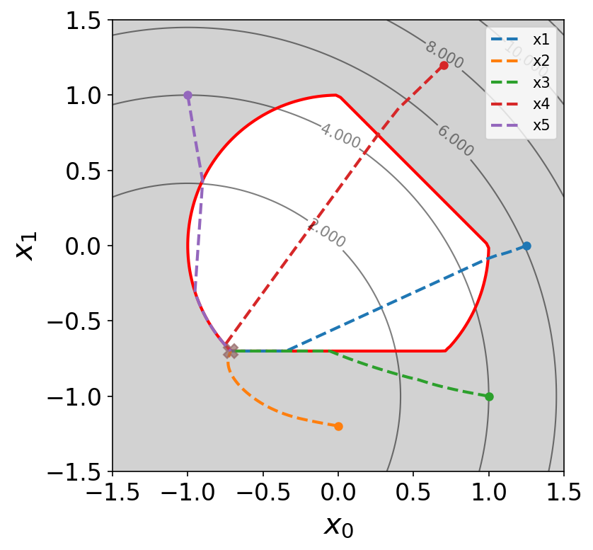
Some optimization trajectories obtained with the open-source implementation of our algorithm on a demonstrative test case.

This algorithm allows, in principle, to solve arbitrary nonlinear constrained optimization problems of the form \[ \newcommand{\x}{{\bf x}} \newcommand{\g}{{\bf g}} \newcommand{\<}{\leqslant} \newcommand{\R}{\mathbb{R}} \newcommand{\h}{{\bf h}} \begin{aligned} \min_{\x\in V}& \quad J(\x)\\ \textrm{s.t.} & \left\{\begin{aligned} \g(\x)&=0\\ \h(\x)&\<0, \end{aligned}\right. \end{aligned} \label{eqn:equation} \tag{1} \] where \(V\) is the optimization set, \(J\,:\,V\to \R\) is the objective function and \(\g\,:\,V\rightarrow \R^p\) and \(\h\,:\,V\rightarrow \R^q\) are respectively the respectively the equality and inequality constraint functionals.

The basis of the method is to solve an Ordinary Differential Equation (so-called ‘’null-space gradient flow’’), \[\begin{equation} \label{eqn:ODE} \dot{x}(t) =-\alpha_J \xi_J(x(t))-\alpha_C\xi_C(x(t)), \end{equation}\] which is able to solve the optimization problem \(\eqref{eqn:equation}\).

The direction \(\xi_J(x(t))\) is called the null space direction, it is the ‘’best’’ locally feasible descent direction for minimizing \(J\) and respecting the constraints. The direction \(\xi_C(x(t))\) is called the range space direction, it makes the violated constraints better satisfied and corrects unfeasible initializations.

Simple illustration of the algorithm

Mathematical definitions of \(\xi_J(x)\) and \(\xi_C(x)\)

The null space direction \(\xi_J(x)\) can be interpreted as a generalization of the gradient in presence of equality and inequality constraints. It is defined as positively proportional to the solution of the following minimization problem: \[\begin{aligned} & \min_{\xi\in V} \quad\mathrm{D}J(x)\xi\\ & \textrm{s.t. } \left\{\begin{aligned} \mathrm{D}\g(x)\xi &= 0\\ \mathrm{D}\h_{\widetilde{I\,}(x)}(x)\xi& \<0\\ ||\xi||_V & \< 1. \end{aligned}\right. \end{aligned} \] where \(\widetilde{I\,}(x)\) is the set of violated or saturated constraints: \[ \widetilde{I\,}(x):=\{i\in \{1,\dots,q\}\,|\, h_i(x)\geqslant 0\}.\] This minimization problem always has a solution. When the number of constraints is not too large, \(\xi_J(x)\) can be computed efficiently by mean of a dual subproblem.

The range space direction \(\xi_C(x)\) is a Gauss-Newton direction for cancelling the violated constraints of \(\widetilde{I\,}(x)\): \[ \newcommand{\CC}{\mathrm{C}} \xi_C(x):=\mathrm{D}\CC_{\widetilde{I\,}(x)}^T(\mathrm{D}\CC_{\widetilde{I\,}(x)} \mathrm{D}\CC_{\widetilde{I\,}(x)}^T)^{-1}\CC_{\widetilde{I\,}(x)}(x), \textrm{ with } \CC_{\widetilde{I\,}}(x):=\begin{bmatrix} \g(x) & \h_{\widetilde{I\,}(x)}(x)\end{bmatrix}^T,\, \h_{\widetilde{I\,}(x)}(x):=(h_i(x))_{i \in \widetilde{I\,}(x)}. \] It is orthogonal to \(\xi_J(x)\) and satisfies \(\mathrm{D}\CC_{\widetilde{I\,}(x)}\xi_C(x)=\CC_{\widetilde{I\,}(x)}(x)\) which entails an exponential decrease of the violation of the constraints at rate at least \(e^{-\alpha_C t}\) for the solution \(x(t)\) of : \[\forall t\geqslant 0,\, \g(x(t))= \g(x(0)) e^{-\alpha_C t}\textrm{ and } \h(x(t)) \< \max(0,\h(x(0))e^{-\alpha_C t}.\]

Demonstration on topology optimization test cases

The algorithm proves very convenient to solve shape optimization test cases, because it does not require to tune meta-parameters (such as penalization parameters) difficult to guess for the user. This algorithm has been used for all our 2-D and 3-D topology optimization test cases.

Let us reproduce below the multiple load bridge test case of our paper [11]. We minimize the volume subject to up to 9 rigidity constraints corresponding to up to 9 different load test cases: \[ \newcommand{\u}{{\bf{u}}} \newcommand{\n}{\bf n} \newcommand{\D}{\mathrm{d}} \renewcommand{\div}{\mathrm{div}} \begin{aligned} \min_{\Gamma} & \quad \int_{\Omega_s} \D x \\ s.t. & \left\{ \begin{aligned} \int_{\Omega_s} Ae(\u_i):e(\u_i)\D x & \< C\textrm{ for }i=1\dots 9 \\ -\div(Ae(\u_i)) & = 0 \textrm{ in }\Omega_s\\ Ae(\u_i)\cdot\n& = \bf g_i \textrm{ on }\Gamma_i\textrm{ for }i=1\dots 9\\ Ae(\u_i)\cdot\n &= 0\textrm{ on } \Gamma\textrm{ for }i=1\dots 9, \end{aligned}\right. \end{aligned}.\] As the number of loads considered increase, the optimization path generates additional supporting bars for rigidity

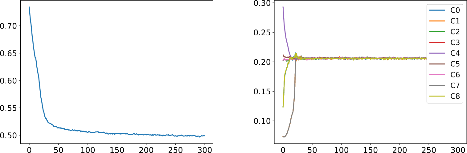
Convergence histories for the nine load test case: the objective function decreases even once the constraints are satisfied.

Null space gradient flows for nonlinear constrained optimization

Simple illustration of the algorithm

Mathematical definitions of \(\xi_J(x)\) and \(\xi_C(x)\)

Demonstration on topology optimization test cases