Lecture 10: LocalGLMnet

Deep Learning for Actuarial Modeling
36th International Summer School SAA
University of Lausanne

Author

Ronald Richman, Salvatore Scognamiglio, Mario V. Wüthrich

Published

September 11, 2025

Abstract

This lecture presents the LocalGLMnet architecture of Richman and Wüthrich (2023). The LocalGLMnet is an extension of a GLM by letting the GLM regression parameters be flexible functions of the covariates.

1 LocalGLMnet architecture

This lecture presents the LocalGLMnet architecture introduced in Richman and Wüthrich (2023b).
The LocalGLMnet architecture extends a GLM with network features by letting the GLM regression parameters be flexible functions (networks) of the covariates. This preserves explainability to some degree, and it also provides universality.
The LocalGLMnet can also be interpreted as a varying coefficient model; see Zhou and Hooker (2022) and Zakrisson and Lindholm (2025).

1.1 Generalized linear model, revisited

We start with the GLM equation.
Assume the covariates $\boldsymbol{X}$ are real-valued.
The GLM equation with link function $g$ is given by \[\boldsymbol{X}~\mapsto~ \mu_{\vartheta}(\boldsymbol{X}) =g^{-1} \left\langle \vartheta, \boldsymbol{X} \right\rangle =g^{-1} \left(\vartheta_0 + \sum_{j=1}^q \vartheta_j \, X_j \right),\] with GLM regression parameter $\vartheta \in {\mathbb R}^{q+1}$.
This GLM regression parameter $\vartheta \in {\mathbb R}^{q+1}$ takes a fixed value.
GLM fitting is done with MLE.
The LocalGLMnet replaces this fixed parameter by a function of ${\boldsymbol{X}}$.

1.2 LocalGLMnet

Select a (deep) multi-output FNN architecture of depth $d\ge 1$ \[ \boldsymbol{z}^{(d:1)}: {\mathbb R}^{q} \to {\mathbb R}^{q},\] with \[ \boldsymbol{X}~\mapsto~ \boldsymbol{z}^{(d:1)}(\boldsymbol{X}) =\left(z_1^{(d:1)}(\boldsymbol{X}), \ldots, z_q^{(d:1)}(\boldsymbol{X}) \right).\]
Note that this multi-output FNN architecture has identical input and output dimension $q$.
We use the output components $(z_j^{(d:1)}(\boldsymbol{X}))_{j=1}^q$ to model flexible GLM parameters.

The LocalGLMnet architecture is defined by \[ \mu_{\vartheta}(\boldsymbol{X}) =g^{-1} \left(\vartheta_0 + \sum_{j=1}^q z_j^{(d:1)}(\boldsymbol{X}) \, X_j \right), \] with a real-valued bias (intercept) parameter $\vartheta_0 \in {\mathbb R}$.
Thus, the GLM parameter $\vartheta$ is replaced by the network outputs $(z_j^{(d:1)}(\boldsymbol{X}))_{j=1}^q$; we call these outputs attention weights.
Locally, these attention weights look like constants (supposed that the FNN is Lipschitz).
Thus, the LocalGLMnet behaves locally like a GLM.
There is a post-hoc explainability method called LIME (local interpretable model-agnostic explanations); Ribeiro, Singh and Guestrin (2016). To some extent, the LocalGLMnet integrates this local interpretability into the model structure.

While we estimated the GLM parameter $\vartheta \in {\mathbb R}^{q+1}$ with MLE, we learn the attention weights $(z_j^{(d:1)}(\boldsymbol{X}))_{j=1}^q$ with SGD.
Because typically the learning data is noisy, the learned attention weights $(z_j^{(d:1)}(\boldsymbol{X}))_{j=1}^q$ will inherit a natural level of fluctuations, which we need to understand to correctly interpret this predictive model.
For smoothing and variable selection one can apply regularization to the attention weights; see Richman and Wüthrich (2023a).

2 Interpretation of attention weights

We focus on the individual terms under the above $j$-summation.

$z^{(d:1)}_j(\boldsymbol{X}) \equiv \vartheta_j \neq 0$: we have a GLM component in this term (this is discussed further below).
$z^{(d:1)}_j(\boldsymbol{X}) \equiv 0$: drop this term; Richman and Wüthrich (2023b) propose an empirical statistical test for dropping terms (this is presented below).
$z^{(d:1)}_j(\boldsymbol{X})=z^{(d:1)}_j(X_j)$: there is no interaction in this term.
Interactions: Consider the gradient \[ \nabla z^{(d:1)}_j(\boldsymbol{X}) = \left( \frac{\partial}{\partial X_1}z^{(d:1)}_j(\boldsymbol{X}),\, \ldots,\, \frac{\partial}{\partial X_q}z^{(d:1)}_j(\boldsymbol{X}) \right) ~\in ~{\mathbb R}^q.\] Non-zero components give interactions (cross-sensitivities).

This all looks very convincing, but there is an issue: the LocalGLMnet regression function lacks identifiability.
Due to the flexibility of large FNNs, we may learn a term that gives us \[ z_j^{(d:1)}(\boldsymbol{X}) \, X_j = X_{j'}, \qquad \text{ for $j'\neq j$.}\]
For this reason, we speak about dropping a ‘term’ and not a ‘covariate component’ in the previous items (1)-(3).
For SGD training of the LocalGLMnet, one needs to initialize the SGD algorithm. We recommend to initialize the network weights such that the SGD algorithm precisely starts in the MLE fitted GLM. Often, this pre-determines the role of all $j$-terms such that one does not encounter the above situation; this initialization is presented below.

3 Variable importance measure

Assume all covariate components are standardized (centered with unit variance), thus, the magnitudes of the attention weights $z_j^{(d:1)}(\boldsymbol{X})$ are directly comparable across all components $1\le j \le q$.
This motivates to consider the variable importance measure \[ \operatorname{VI}_j = \frac{1}{n} \,\sum_{i=1}^n \left| z_j^{(d:1)}(\boldsymbol{X}_i)\right|.\]
If this value is very small, the empirical test of Richman and Wüthrich (2023a) gives support to the null-hypothesis of dropping this term and, obviously, if $\operatorname{VI}_j$ is large it has a big impact on the regression function; this is similar to the likelihood ratio test (LRT) for GLMs.
We describe this variable importance test below.

4 LocalGLMnet example

4.1 LocalGLMnet example

We illustrate the LocalGLMnet architecture on the French MTPL claims frequency data. We start with a Poisson GLM example which allows us to compare the attention weights of the LocalGLMnet to the GLM parameters.

Load the French MTPL data (with entity embeddings)

load(file="../Data/freMTPL2freqEmb.rda")
dat <- freMTPL2freqEmb     # this data contains the entity embeddings

Simplification

To avoid any complications with categorical covariates, we use the two-dimensional entity embeddings of the categorical covariates obtained from the plain-vanilla FNN from the previous lectures.

One could also implement categorical covariates by one-hot encoding, but then statistical testing becomes more difficult, and one should rather use methods like group LASSO regularization; see Richman and Wüthrich (2023a).
Alternatively, categorical covariates could only enter the attention weights, for modeling the continuous covariates only; and there are many other alternatives.

Covariate pre-processing

# function for standardization
PreProcess.Continuous <- function(var1, dat2){
   names(dat2)[names(dat2) == var1]  <- "V1"
   dat2$X <- as.numeric(dat2$V1)
   dat2$X <- (dat2$X-mean(dat2$X))/sd(dat2$X)
   names(dat2)[names(dat2) == "V1"]  <- var1
   names(dat2)[names(dat2) == "X"]  <- paste(var1,"X", sep="")
   dat2
   }

We only have continuous covariates in this example because we work with the entity embeddings of the categorical covariates.
Again, the learning and test sample should use the identical standardization, and the parameters need to be stored for the consideration of new data.

# pre-processing all covariates
Features.PreProcess <- function(dat2){
   dat2 <- PreProcess.Continuous("Area", dat2)
   dat2 <- PreProcess.Continuous("VehPower", dat2)
   dat2$VehAge <- pmin(dat2$VehAge,20)
   dat2 <- PreProcess.Continuous("VehAge", dat2)
   dat2$DrivAge <- pmin(dat2$DrivAge,90)
   dat2 <- PreProcess.Continuous("DrivAge", dat2)
   dat2$BonusMalus <- pmin(dat2$BonusMalus,150)
   dat2 <- PreProcess.Continuous("BonusMalus", dat2)
   dat2 <- PreProcess.Continuous("VehBrandEmb1", dat2)
   dat2 <- PreProcess.Continuous("VehBrandEmb2", dat2)
   dat2 <- PreProcess.Continuous("VehGas", dat2)
   dat2$Density <- round(log(dat2$Density),2)
   dat2 <- PreProcess.Continuous("Density", dat2)
   dat2 <- PreProcess.Continuous("RegionEmb1", dat2)
   dat2 <- PreProcess.Continuous("RegionEmb2", dat2)}
dat <- Features.PreProcess(dat)

Add an unassociated covariate

# we add a purely random component for significance testing 
set.seed(100)
dat$RandN  <- rnorm(n=nrow(dat), mean=0, sd=1)
dat$RandNX <- dat$RandN

## learn and test sample partition
learn <- dat[which(dat$LearnTest=='L'),]
test  <- dat[which(dat$LearnTest=='T'),]

We add a purely random and independent component to the covariates (being centered and with unit variance as all other covariate components).
This random component will assess the level of fluctuations in the attention weights that can be explained by pure randomness (noise).
This will allow us to perform a test for variable selection.

GLM on the continuous (normalized) covariates

d.glm <- glm(ClaimNb ~ AreaX + VehPowerX + VehAgeX + DrivAgeX + BonusMalusX + VehGasX + DensityX + VehBrandEmb1X + VehBrandEmb2X + RegionEmb1X + RegionEmb2X + RandNX,
            data=learn, offset=log(Exposure), family=poisson())
#
Poisson.Deviance <- function(pred, obs, weight){ 100*2*(sum(pred)-sum(obs)+sum(log((obs/pred)^(obs))))/sum(weight) }
#
learn$GLM <- fitted(d.glm)
test$GLM  <- predict(d.glm, newdata=test, type="response")
#
round(c(Poisson.Deviance(learn$GLM, learn$ClaimNb, learn$Exposure), Poisson.Deviance(test$GLM, test$ClaimNb, test$Exposure)), 3)

[1] 45.761 45.629

...
Coefficients:
               Estimate Std. Error  z value Pr(>|z|)    
(Intercept)   -2.668685   0.007033 -379.443  < 2e-16 ***
AreaX          0.055287   0.027562    2.006  0.04487 *  
VehPowerX      0.065128   0.006725    9.684  < 2e-16 ***
VehAgeX       -0.096715   0.007489  -12.914  < 2e-16 ***
DrivAgeX       0.082829   0.006894   12.015  < 2e-16 ***
BonusMalusX    0.415996   0.005702   72.957  < 2e-16 ***
VehGasX       -0.087107   0.006668  -13.064  < 2e-16 ***
DensityX       0.083135   0.027278    3.048  0.00231 ** 
VehBrandEmb1X  0.118213   0.014395    8.212  < 2e-16 ***
VehBrandEmb2X  0.030369   0.014746    2.059  0.03946 *  
RegionEmb1X   -0.089435   0.007356  -12.158  < 2e-16 ***
RegionEmb2X    0.016721   0.007916    2.112  0.03466 *  
RandNX        -0.003710   0.006502   -0.571  0.56832    
---
Signif. codes:  0 '***' 0.001 '**' 0.01 '*' 0.05 '.' 0.1 ' ' 1

(Dispersion parameter for poisson family taken to be 1)

    Null deviance: 153852  on 610205  degrees of freedom
Residual deviance: 147529  on 610193  degrees of freedom
AIC: 193207

Number of Fisher Scoring iterations: 6
...

Interpretation of GLM results

Though we did not perform a proper covariate pre-processing for GLMs, the GLM results are surprisingly good; a properly pre-processed GLM has an out-of-sample loss of 45.435 (vs. 45.629 in the above GLM).
The above component-wise Wald tests (drop1 analysis) only question the inclusion of RandNX (the purely random covariate).
AreaX could be questioned ($p$-value of 4.5%), and two embedding components have $p$-values between 3.5% and 4%; note that this does not tell us too much, yet, because we did not pay any attention to suitable functional forms in the covariates.

LocalGLMnet architecture of depth 3

LocalGLMnet <- function(seed, q0){
    tf$keras$backend$clear_session()
    set.seed(seed)
    set_random_seed(seed)
    Design  <- layer_input(shape = c(q0[1]), dtype = 'float32')
    Volume  <- layer_input(shape = c(1),     dtype = 'float32')
    Attention = Design %>%
          layer_dense(units=q0[2], activation='tanh') %>%
          layer_dense(units=q0[3], activation='tanh') %>%
          layer_dense(units=q0[4], activation='tanh') %>%
          layer_dense(units=q0[1], activation='linear', name='Attention')
    # careful: Keras 2 axes=1; Keras 3 axes=2
    LocalGLM = list(Design, Attention) %>% layer_dot(axes=1) %>%
                    layer_dense(units=1, activation='exponential')
    Response = list(LocalGLM, Volume) %>% layer_multiply()
    keras_model(inputs = c(Design, Volume), outputs = c(Response)) 
    }

Prepare data for LocalGLMnet fitting

# prepare data for LocalGLMnet fitting
names0 <- c("Area", "VehPower", "VehAge", "DrivAge", "BonusMalus", "VehGas", "Density", "VehBrandEmb1", "VehBrandEmb2", "RegionEmb1", "RegionEmb2", "RandN")
#
Xlearn  <- as.matrix(learn[, paste0(names0,"X")])  
Xtest   <- as.matrix(test[, paste0(names0,"X")])   
Vlearn  <- as.matrix(learn$Exposure)
Vtest   <- as.matrix(test$Exposure)
Ylearn  <- as.matrix(learn$ClaimNb)
Ytest   <- as.matrix(test$ClaimNb)
# 
q00 <- c(length(names0), c(20,15,10))    # select architecture
seed <- 100
model <- LocalGLMnet(seed, q00)

...
 Layer (type)           Output Shape            Param   Connected to            
                                                 #                              
================================================================================
 input_1 (InputLayer)   [(None, 12)]            0       []                      
 dense_2 (Dense)        (None, 20)              260     ['input_1[0][0]']       
 dense_1 (Dense)        (None, 15)              315     ['dense_2[0][0]']       
 dense (Dense)          (None, 10)              160     ['dense_1[0][0]']       
 Attention (Dense)      (None, 12)              132     ['dense[0][0]']         
 dot (Dot)              (None, 1)               0       ['input_1[0][0]',       
                                                         'Attention[0][0]']     
 dense_3 (Dense)        (None, 1)               2       ['dot[0][0]']           
 input_2 (InputLayer)   [(None, 1)]             0       []                      
 multiply (Multiply)    (None, 1)               0       ['dense_3[0][0]',       
                                                         'input_2[0][0]']       
================================================================================
Total params: 869 (3.39 KB)
Trainable params: 869 (3.39 KB)
Non-trainable params: 0 (0.00 Byte)
________________________________________________________________________________
...

Initialize with GLM parameters

# initialize with GLM weights
w0       <- get_weights(model)
w0[[7]]  <- array(0, dim=dim(w0[[7]]))
w0[[8]]  <- array(d.glm$coefficients[2:(length(names0)+1)], dim=dim(w0[[8]]))    # these biases are set to the GLM parameters
w0[[9]]  <- array(1, dim=dim(w0[[9]]))
w0[[10]] <- array(d.glm$coefficients[1], dim=dim(w0[[10]]))
set_weights(model, w0)

# check correctness of this GLM initialization
learn.GLM <- model %>% predict(list(Xlearn, Vlearn), batch_size=10^6)
test.GLM  <- model %>% predict(list(Xtest, Vtest), batch_size=10^6)
(loss.GLM <- round(c(Poisson.Deviance(learn.GLM, Ylearn, Vlearn), Poisson.Deviance(test.GLM, Ytest, Vtest)), 3))

[1] 45.761 45.629

LocalGLMnet fitting

## define callback for early stopping
if (!dir.exists("./Networks")){dir.create("./Networks")}
path1 <- paste0("./Networks/LocalGLMnet1",seed,".weights.h5")
CBs <- callback_model_checkpoint(path1, monitor = "val_loss", verbose = 0,  save_best_only = TRUE, save_weights_only = TRUE)

## compile with Poisson deviance loss and nadam optimizer
model %>% compile(loss = 'poisson', optimizer = 'nadam')
##
fit <- model %>% fit(list(Xlearn, Vlearn),  Ylearn,
                    validation_split=0.1, batch_size=5000, epochs=200, verbose=0, callbacks=CBs)
# early stopping time
which.min(fit[[2]]$val_loss)

[1] 38

LocalGLMnet results

# load early stopping solution
model$load_weights(path1)
w2 <- get_weights(model)

# cumpute the mean estimates
learn$LocalGLMnet <- model %>% predict(list(Xlearn, Vlearn), batch_size=10^6)
test$LocalGLMnet <- model %>% predict(list(Xtest, Vtest), batch_size=10^6)

# in-sample and out-of-sample losses
rbind(round(loss.LocalGLMnet <- c(Poisson.Deviance(learn$LocalGLMnet, Ylearn, Vlearn), Poisson.Deviance(test$LocalGLMnet, Ytest, Vtest)), 3), loss.GLM)

                   [,1]   [,2]
loss.LocalGLMnet 44.907 45.060
loss.GLM         45.761 45.629

4.2 Comparison to the previous results

model	in-sample loss	out-of-sample loss	balance (in %)
Poisson null model	47.722	47.967	7.36
Poisson GLM	45.585	45.435	7.36
Poisson FNN	44.846	44.925	7.17
embedding FNN	45.030	44.948	7.16
LocalGLMnet	44.907	45.060	7.26

The LocalGLMnet seems slightly worse. This is also impacted by adding the pure noise term RandN (more over-fitting potential), which we need below for variable selection. For fitting the final model, this pure noise term should be dropped and the model re-fitted.
Standard deviations in in-sample and out-of-sample losses were 0.053 and 0.033, respectively (from ensembling).

4.3 Illustration of LocalGLMnet results

## extract the attention weight module
aa <- keras_model(inputs=model$input, outputs=get_layer(model, 'Attention')$output)

## compute the attention weights
Aa.x <- data.frame(aa %>% predict(list(Xtest, Vtest), batch_size=10^6))
names(Aa.x) <- names0              # label the columns
Aa.x <- Aa.x * as.numeric(w2[[9]]) # account for overall scaling of output

## summary statistics of the purely random component
c(mean(Aa.x[,"RandN"]), sdN <- sd(Aa.x[,"RandN"]))

[1] -0.01904157  0.03891009

$\Longrightarrow$ This is the bias and uncertainty that can be explained by pure noise.

Boxplot of resulting attention weights (of all terms)

The confidence bounds are determined by the results of RandN.
The orange area gives the inter-quartile area (careful, this does not consider the bias of RandN).
The red lines give the 99% significance bounds.
RandN has clearly the smallest boxplot, the boxplot of Area is also small, but not centered.
This plot suggest to keep all components.
In the next plots we show the individual (out-of-sample) attention weights $(z_j^{(d:1)}(\boldsymbol{X}_t))_{t=1}^m$ of selected covariate components $j$; the $y$-scale is always the same in these plots.

This calibrates the drop1 test.

The vertical spreading/scattering indicates interactions.

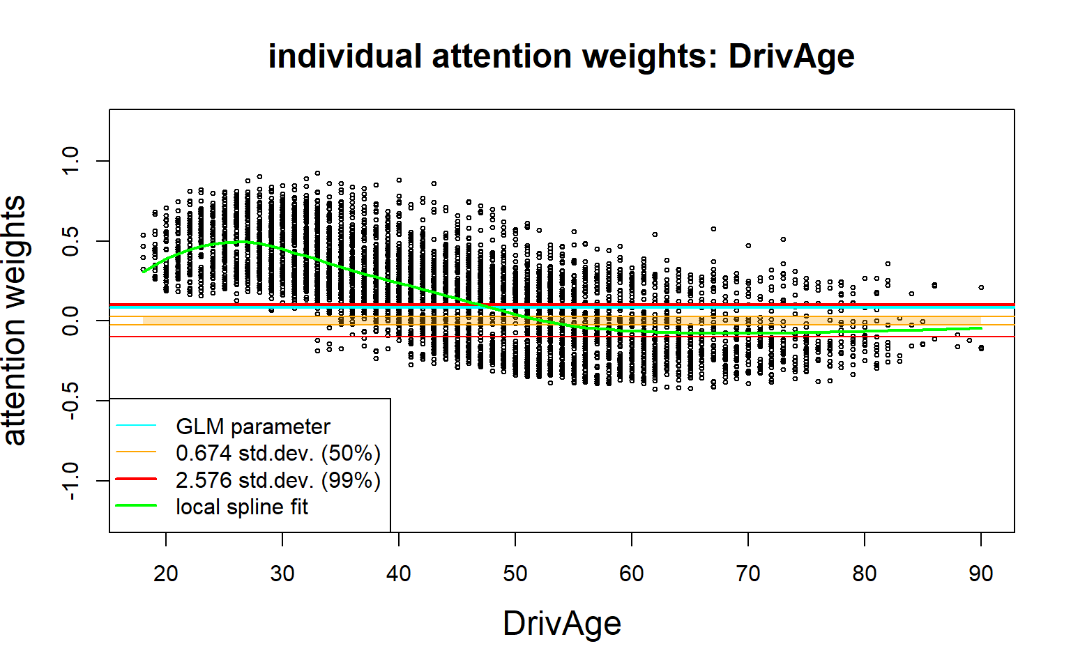
The vertical spreading/scattering indicates interactions.

This neglects collinearity with Density; the vertical scatter exceeds the confidence bounds.

Variable importance measure

# compute and order for variable importance indices
VI <- abs(Aa.x)
VI <- colMeans(VI)
VI.names <- names0[(order(VI))]
VI <- VI[(order(VI))]

# plot variable importance
par(mar=c(5.1,7,4.1,2.1)) # increase y-axis margin.
barplot(t(VI), las=1, beside=TRUE, col=c("red"), names.arg=VI.names, main=list("importance measure", cex=1.5), horiz=TRUE)
abline(v=0)
abline(v=mean(VI[1:1]), col="blue", lwd=2)
abline(v=c(0:10)*0.1, lty=2)
par(mar=c(5.1,4.1,4.1,2.1))

Gradients of interactions

# to make gradient computations easier we drop the volumes
LocalGLMnet.NoVolume <- function(seed, q0){
  tf$keras$backend$clear_session()
  set.seed(seed)
  set_random_seed(seed)
  Design  <- layer_input(shape = c(q0[1]), dtype = 'float32')
  Attention = Design %>%
    layer_dense(units=q0[2], activation='tanh') %>%
    layer_dense(units=q0[3], activation='tanh') %>%
    layer_dense(units=q0[4], activation='tanh') %>%
    layer_dense(units=q0[1], activation='linear', name='Attention')
  # careful: Keras 2 axes=1; Keras 3 axes=2
  LocalGLM = list(Design, Attention) %>% layer_dot(axes=1) %>%
    layer_dense(units=1, activation='exponential')
  keras_model(inputs = Design, outputs = c(LocalGLM))}

Calibrate this architecture to the previous LocalGLMnet.

# set the model back to the fitted weights
model <- LocalGLMnet.NoVolume(seed, q00)
set_weights(model, w2)

# restore the attention weights
zz <- keras_model(inputs=model$input, outputs=get_layer(model, 'Attention')$output)

This is are the attention weights $\boldsymbol{z}^{(d:1)}(\boldsymbol{X})=(z_1^{(d:1)}(\boldsymbol{X}), \ldots, z_q^{(d:1)}(\boldsymbol{X}))^\top$.

Gradient computations for a fixed component $\boldsymbol{X}\mapsto z_j^{(d:1)}(\boldsymbol{X})$.

# function to compute the gradients for component output_index
compute_gradient_wrt_inputs <- function(model, inputs, output_index) {
    inputs_tensor <- tf$convert_to_tensor(inputs, dtype = tf$float32)
    batch_size <- dim(inputs_tensor)[1]
    input_dim <- dim(inputs_tensor)[2]
    gradients <- array(0, dim = c(batch_size, input_dim))
    with(tf$GradientTape() %as% tape, {
      tape$watch(inputs_tensor)
      predictions <- model(inputs_tensor)
      output_component <- predictions[, output_index]
    })
    grad <- tape$gradient(output_component, inputs_tensor)
    return(as.array(grad))
  }

# Compute the gradients for the term 'driver age'
x <- 4
gradients <- compute_gradient_wrt_inputs(zz, Xtest, x)

# fit splines to get the trends
kk <- sort(unique(test[,names0[x]]))
#
for (i in c(1:length(names0))){
   spline0 <- predict(locfit(gradients[,i] ~ test[,names0[x]], alpha=0.3, deg=2), newdata=kk)
   if (i==1){
       spline1 <- spline0
       }else{
       spline1 <- rbind(spline1,spline0)
       }}

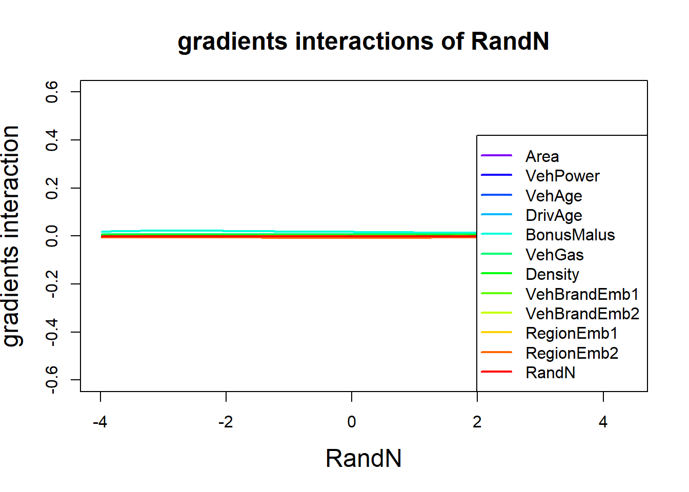
These spline smoothed gradients are plotted in the next graph.

We observe significant interactions between DrivAge and the pair (BonusMalus and Density); note that we did not normalize the quantities.
The second derivative w.r.t. DrivAge is non-zero which says that we cannot have a GLM term in DrivAge.
In an attempt to imprive a GLM, we model DrivAge categorically (as has been done above), and we can manually add interaction terms between DrivAge, BonusMalus and Density to the GLM regression function; an example with interactions is given in Listing 5.8 of Wüthrich and Merz (2023).
The next graph verifies that RandN is independent from any other variable, in particular, the response variable.

Copyright

© The Authors
This notebook and these slides are part of the project “AI Tools for Actuaries”. The lecture notes can be downloaded from:

https://papers.ssrn.com/sol3/papers.cfm?abstract_id=5162304

$\,$

This material is provided to reusers to distribute, remix, adapt, and build upon the material in any medium or format for noncommercial purposes only, and only so long as attribution and credit is given to the original authors and source, and if you indicate if changes were made. This aligns with the Creative Commons Attribution 4.0 International License CC BY-NC.

References

Ribeiro, M.T., Singh, S. and Guestrin, C. (2016) “‘Why should I trust you?’: Explaining the predictions of any classifier,” in Proceedings of the 22nd ACM SIGKDD international conference on knowledge discovery and data mining, pp. 1135–1144. Available at: https://arxiv.org/abs/1602.04938.

Richman, R. and Wüthrich, M.V. (2023a) “LASSO regularization within the LocalGLMnet architecture,” Advances in Data Analysis and Classification, 17(4), pp. 951–981. Available at: https://link.springer.com/article/10.1007/s11634-022-00529-z.

Richman, R. and Wüthrich, M.V. (2023b) “LocalGLMnet: Interpretable deep learning for tabular data,” Scandinavian Actuarial Journal, 2023(1), pp. 71–95. Available at: https://doi.org/10.1080/03461238.2022.2081816.

Wüthrich, M.V. and Merz, M. (2023) Statistical foundations of actuarial learning and its applications. Springer. Available at: https://doi.org/10.1007/978-3-031-12409-9.

Zakrisson, H. and Lindholm, M. (2025) “A tree-based varying coefficient model,” Computational Statistics, 0(0), pp. 0–0. Available at: https://doi.org/10.1007/s00180-025-01603-8.

Zhou, Y. and Hooker, G. (2022) “Decision tree boosted varying coefficient models,” Data Mining and Knowledge Discovery, 36(6), pp. 2237–2271. Available at: https://doi.org/10.1007/s10618-022-00863-y.