load(file="../Data/freMTPL2freqClean.rda")
dat <- freMTPL2freqClean
head(dat[,c(1:11,13)])Lecture 1: Use Case - MTPL data
Deep Learning for Actuarial Modeling
36th International Summer School SAA
University of Lausanne
36th International Summer School SAA
University of Lausanne
Abstract
We start by discussing a car insurance pricing problem which is at the core of actuarial modeling. This example will serve us as a running example through many of the chapters of our lectures.
1 Actuarial modeling
We start with a car insurance pricing problem.
This initial example will mostly be empirical.
It considers the familiar French motor third party liability (MTPL) claims dataset freMTPL2freq of Dutang, Charpentier and Gallic (2024).
Generally, raw data needs data cleaning, e.g., correcting for data errors, inputting missing values, merging partial information, etc. The data presented below has already been cleaned; for details see Appendix B in Wüthrich and Merz (2023).
1.1 Load and illustrate the French MTPL data
- The (cleaned) data contains the following variables:
- ‘IDpol’ is a unique policy identifier
- ‘Exposure’ is the time exposure (in yearly units)
- ‘Area’ is an area code (ordinal categorical)
- ‘VehPower’ is the power of the vehicle
- ‘VehAge’ is the age of the vehicle
- ‘DrivAge’ is the age of the policyholder
- ‘BonusMalus’ is the bonus-malus level of the policyholder
- ‘VehBrand’ indicates the vehicle brand (categorical)
- ‘VehGas’ indicates the gasoline type (categorical)
- ‘Density’ is the population density at the living place of the policyholder
- ‘Region’ gives the French department of the license plate (categorical)
- ‘ClaimNb’ gives the observed number of claims
    IDpol Exposure Area VehPower VehAge DrivAge BonusMalus VehBrand  VehGas
1 4156370     0.06    D        6      6      20        100       B2 Regular
2 4006798     0.29    E        6      7      29         59      B12  Diesel
3 6084964     0.46    C        7     10      27         68       B1  Diesel
4 2228865     0.08    D        4     15      34         50       B2 Regular
5 4141911     1.00    A        5     22      44         50       B3  Diesel
6 1103292     0.60    C        5      2      25         90       B5 Regular
  Density Region ClaimNb
1     525    R82       0
2    2498    R72       0
3     123    R82       0
4    1109    R24       0
5      34    R72       0
6     129    R41       0
For simplicity, we focus on the claims counts ‘ClaimNb’; there would also be data available with claim amounts.
1.2 Claims count modeling and frequencies
The above portfolio has \(n=678,007\) insurance policyholders \(i \in \{1, \ldots, n\}\).
These policyholders are characterized by covariates \(\boldsymbol{X}_i\) describing their policy features such as the age of the car or the vehicle brand.
For each policyholder we have observed their numbers of claims \(N_i \ge 0\) within the given calendar year.
The time exposures \(v_i \in (0, 1]\) give the proportions of the calendar year during which the policies have been active (exposed).
To account for the different time exposures, one typically studies the claims frequencies \[ Y_i = N_i/v_i. \]
The general goal of actuaries is to predict the (future) claims frequencies \(Y_i\) as accurately as possible.
These predictions take into account all available/relevant policyholder information \(\boldsymbol{X}_i\), as this information may reveal structural differences in their propensity to claims.
Predictors are typically computed by conditional means \[ \mu(\boldsymbol{X}_i)=\mathbb{E}\left[Y_i \left| \boldsymbol{X}_i\right]\right. .\]
- \(\mathbb{E}[Y_i | \boldsymbol{X}_i]\) is the expected claim of a policyholder with covariates \(\boldsymbol{X}_i\).
- \(\boldsymbol{X} \mapsto \mu(\boldsymbol{X})\) models these expected claims as a regression function of the policyholder covariates \(\boldsymbol{X}\).
For actuarial pricing, one aims to find an accurate regression function \[\boldsymbol{X} \mapsto \mu(\boldsymbol{X}).\]
1.3 Regression modeling
In general, the true data generating model is unknown.
Therefore, one cannot compute the regression function \(\boldsymbol{X} \mapsto \mu(\boldsymbol{X})\), but one rather needs to estimate it from past data \[ {\cal L} = \left(Y_i, \boldsymbol{X}_i, v_i\right)_{i=1}^n.\]
\({\cal L}\) is called learning sample because it is used to learn the unknown regression function \(\boldsymbol{X} \mapsto \mu(\boldsymbol{X})\).
Before solving this estimation/learning problem, we empirically study the available data \({\cal L} = (Y_i, \boldsymbol{X}_i, v_i)_{i=1}^n\). This is crucial to fully understand the problem and to select a suitable class of candidate regression models.
2 Empirical data analysis
Before trying to find an appropriate regression function \(\boldsymbol{X}\mapsto \mu(\boldsymbol{X})\), we empirically analyze the learning sample \({\cal L}\).
Such an empirical analysis of the learning sample \({\cal L}\) includes different sample statistics as well as visualizations of the data.
For simplicity, we only consider two covariates in this preliminary analysis: ‘DrivAge’ and ‘Density’. In later examples, all covariates are considered.
We start by classifying the policies w.r.t. their numbers of claims.
library(arrow)
library(tidyverse)
#
dat %>% group_by(ClaimNb) %>% summarize(Exposure = sum(Exposure))
ClaimNb Exposure
1 0 341090
2 1 16315
3 2 909
4 3 42
5 4 2
6 5 1The above table shows that the majority of insurance policies does not suffer any claims.
The empirical claims frequency is \(\sum_{i=1}^n N_i/\sum_{i=1}^n v_i=7.36\%\).
In machine learning, this is called a class imbalance problem.
In actuarial modeling, this is just the typical problem actuaries have to solve, i.e., actuaries try to find systematic structure in data in which claims are rare events.
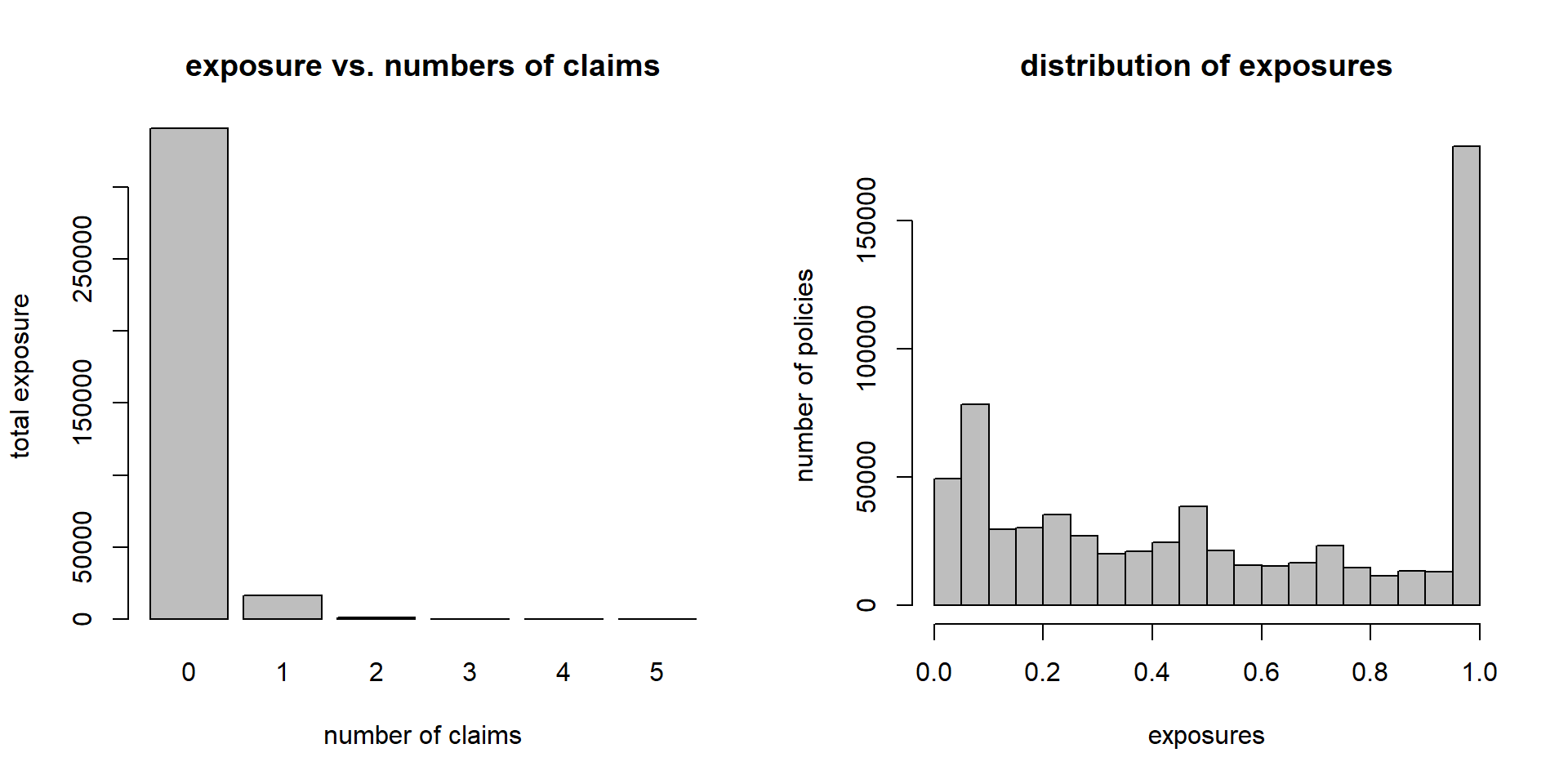
(lhs): class imbalance problem mentioned above.
(rhs): distribution of the exposures \((v_i)_{i=1}^n\), roughly 25% of the policies have a full-year exposure \(v_i=1\) in this data.
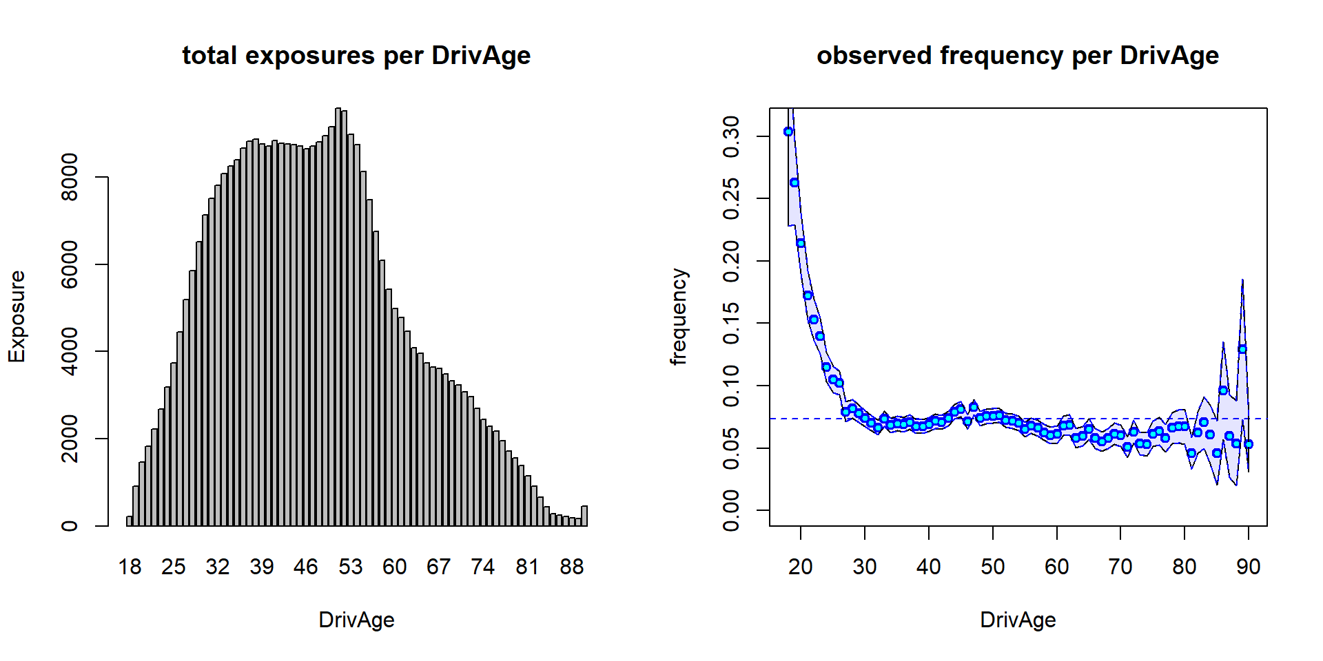
(lhs): total exposure \(\sum_i v_i \mathbf{1}_{\{{\rm age_i}={\rm age}\}}\) per age class.
(rhs): empirical frequency \(\sum_i N_i \mathbf{1}_{\{{\rm age_i}={\rm age}\}}/\sum_i v_i \mathbf{1}_{\{{\rm age_i}={\rm age}\}}\) per age class; confidence bounds correspond to 2 std in a Poisson model.
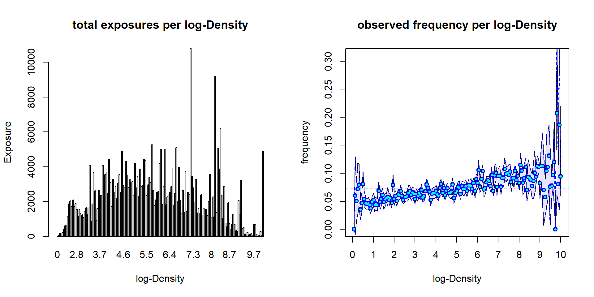
(lhs): total exposure \(\sum_i v_i \mathbf{1}_{\{{\rm LD_i}={\rm LD}\}}\) per log-Density (class LD).
(rhs): empirical frequency \(\sum_i N_i \mathbf{1}_{\{{\rm LD_i}={\rm LD}\}}/\sum_i v_i \mathbf{1}_{\{{\rm LD_i}={\rm LD}\}}\) per log-Density; confidence bounds correspond to 2 std in a Poisson model.
The previous plots show the marginal distributions of the claims.
Generally, covariates interact so that one cannot simply multiply marginal observations to receive the correct prices.
E.g.: Young drivers may all live in the highly-populated cities, and the high frequencies at younger ages and in densely populated areas are driven by the same risk factor. Multiplying marginals will, thus, result in a double penalty of the same risk factor.
For this reason, we need to understand the multivariate picture to receive a good pricing functional \(\boldsymbol{X}\mapsto \mu(\boldsymbol{X})\).
I.e., we need to estimate \(\mu(\boldsymbol{X})\) jointly in the two components of \(\boldsymbol{X}=(X_1,X_2)^\top\), and not marginally.
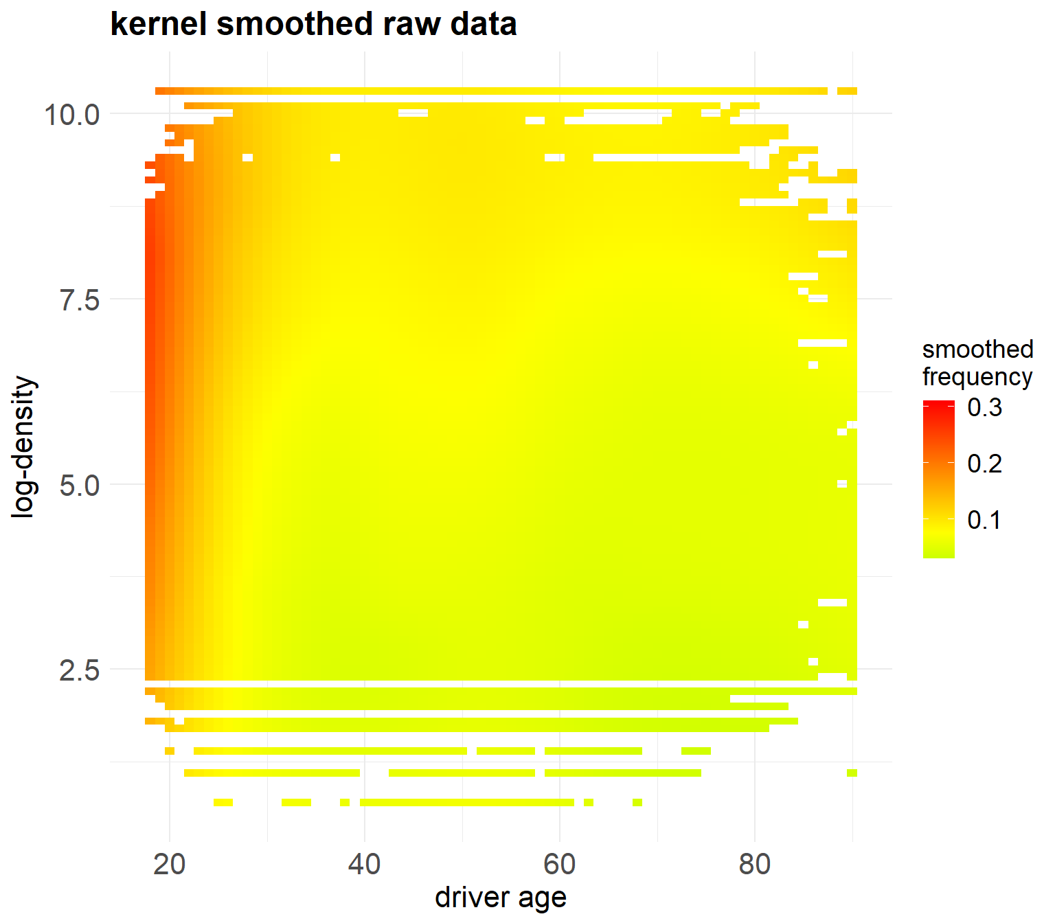
The above heatmap shows the empirical frequency as a function of the two covariates ‘DrivAge’ and ‘log-Density’.
The empirical data has been smoothed with the kernel smoothing method called ‘loess’ (locally estimated scatterplot smoothing).
The colored dots show the loess results in the covariate combinations that exist in our portfolio, and the white space corresponds to covariate combinations that are not available in our portfolio.
The coloring shows quite some non-linear structure in the covariate components.
3 A generalized linear model example
We start with a generalized linear model (GLM) for the regression functional \(\boldsymbol{X}\mapsto \mu(\boldsymbol{X})\).
The underlying mathematical theory is going to be presented in careful detail in later notebooks.
The most simple GLM setting is \[ \boldsymbol{X}\mapsto \mu(\boldsymbol{X}) = \exp \left(\beta_0 + \beta_1 X_1+ \beta_2 X_2\right),\] for \(\boldsymbol{X}=(X_1,X_2)=(\text{DrivAge}, \text{log-Density})\) and parameter \((\beta_0,\beta_1,\beta_2)\).
### Model GLM 1 (Poisson for counts with offsets)
d.glm1 <- glm(ClaimNb ~ DrivAge + lDensity, data=dat, offset=log(Exposure), family=poisson())
#
dat$GLM1 <- fitted(d.glm1)
summary(d.glm1)
Call:
glm(formula = ClaimNb ~ DrivAge + lDensity, family = poisson(),
    data = dat1, offset = log(Exposure))

Coefficients:
              Estimate Std. Error z value Pr(>|z|)
(Intercept) -2.7811529  0.0298084  -93.30   <2e-16 ***
DrivAge     -0.0097160  0.0004414  -22.01   <2e-16 ***
lDensity     0.1023950  0.0032929   31.10   <2e-16 ***
---
Signif. codes:  0 '***' 0.001 '**' 0.01 '*' 0.05 '.' 0.1 ' ' 1

(Dispersion parameter for poisson family taken to be 1)

    Null deviance: 9169.3  on 5988  degrees of freedom
Residual deviance: 7647.9  on 5986  degrees of freedom
AIC: 22487

Number of Fisher Scoring iterations: 5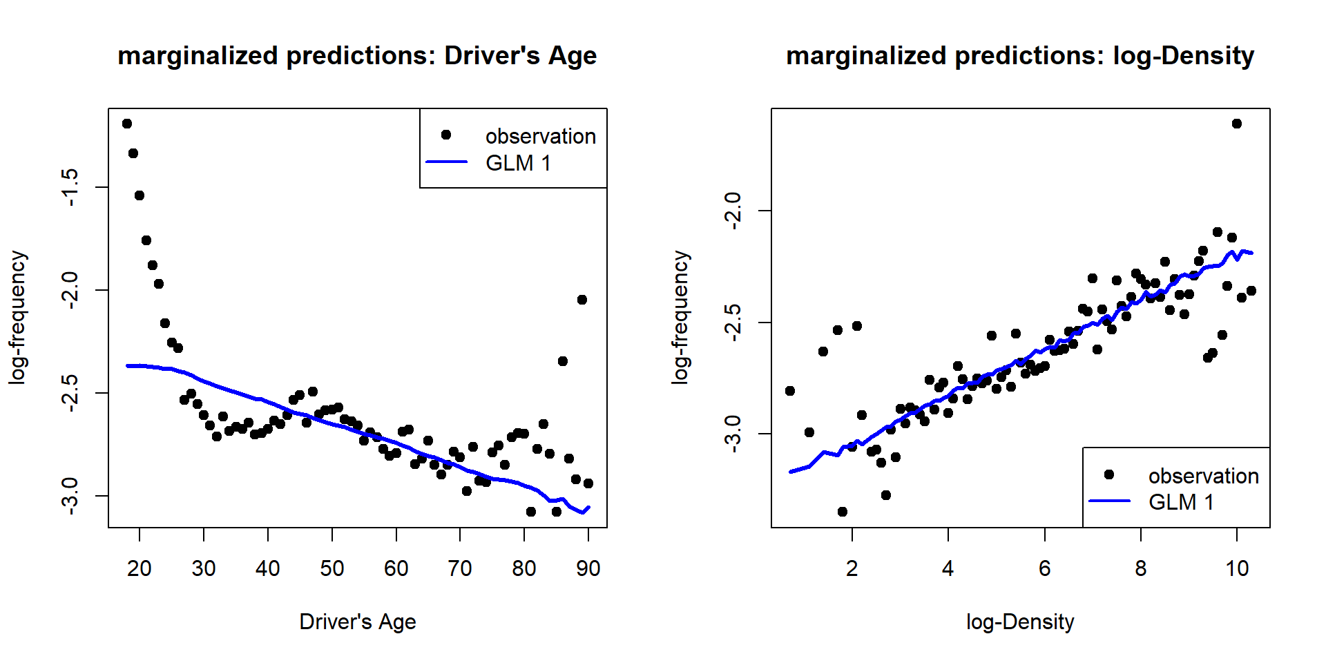
- Obviously, the driver’s age variable does not fit the observed data, as this GLM is not able to model the non-monotone structure.
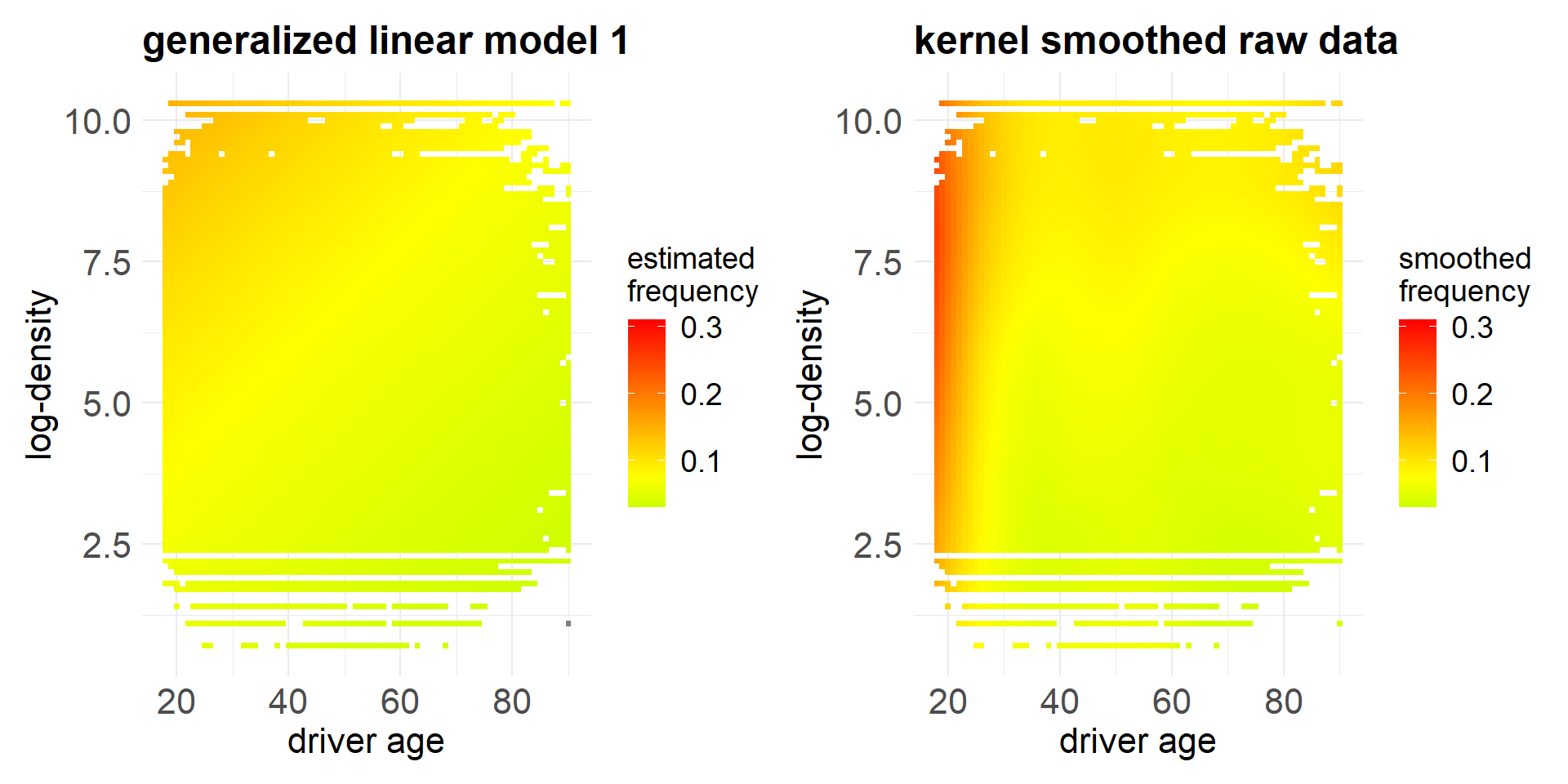
- The heatmap confirms that this GLM is not able to reflect the observed data.
Usually, in case of non-monotone behavior, one builds categorical classes.
We build age classes as follows (which are then implemented by dummy coding).
### Model GLM 2
dat$DrivAgeGLM    <- as.factor(cut(dat$DrivAge, c(18,20,25,30,40,50,70,101), labels = c("18-20", "21-25", "26-30", "31-40", "41-50", "51-70", "71+"), include.lowest = TRUE))
#
# Poisson GLM with (canonical) log-link
d.glm2 <- glm(ClaimNb ~ DrivAgeGLM + lDensity, data=dat, offset=log(Exposure), family=poisson())
#
dat$GLM2 <- fitted(d.glm2)- This estimates an individual regression parameter \(\beta_j\) for each age class.
Call:
glm(formula = ClaimNb ~ DrivAgeGLM + lDensity, family = poisson(),
    data = dat1, offset = log(Exposure))

Coefficients:
                 Estimate Std. Error z value Pr(>|z|)
(Intercept)     -2.047914   0.044931  -45.58   <2e-16 ***
DrivAgeGLM21-25 -0.627963   0.046706  -13.45   <2e-16 ***
DrivAgeGLM26-30 -1.109290   0.045196  -24.54   <2e-16 ***
DrivAgeGLM31-40 -1.261688   0.042354  -29.79   <2e-16 ***
DrivAgeGLM41-50 -1.165688   0.042086  -27.70   <2e-16 ***
DrivAgeGLM51-70 -1.298062   0.041879  -31.00   <2e-16 ***
DrivAgeGLM71+   -1.380917   0.047348  -29.16   <2e-16 ***
lDensity         0.104394   0.003301   31.62   <2e-16 ***
---
Signif. codes:  0 '***' 0.001 '**' 0.01 '*' 0.05 '.' 0.1 ' ' 1

(Dispersion parameter for poisson family taken to be 1)

    Null deviance: 9169.3  on 5988  degrees of freedom
Residual deviance: 6858.0  on 5981  degrees of freedom
AIC: 21707

Number of Fisher Scoring iterations: 5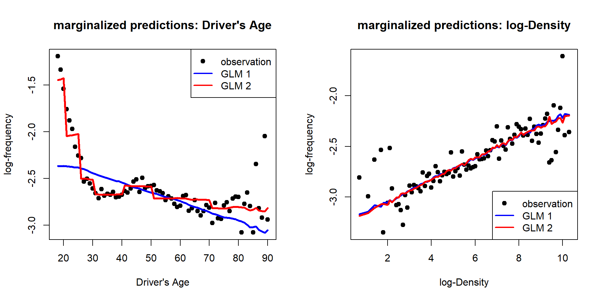
This second GLM with categorical age classes fits the data better.
Because of the log-link choice, it has a multiplicative structure.
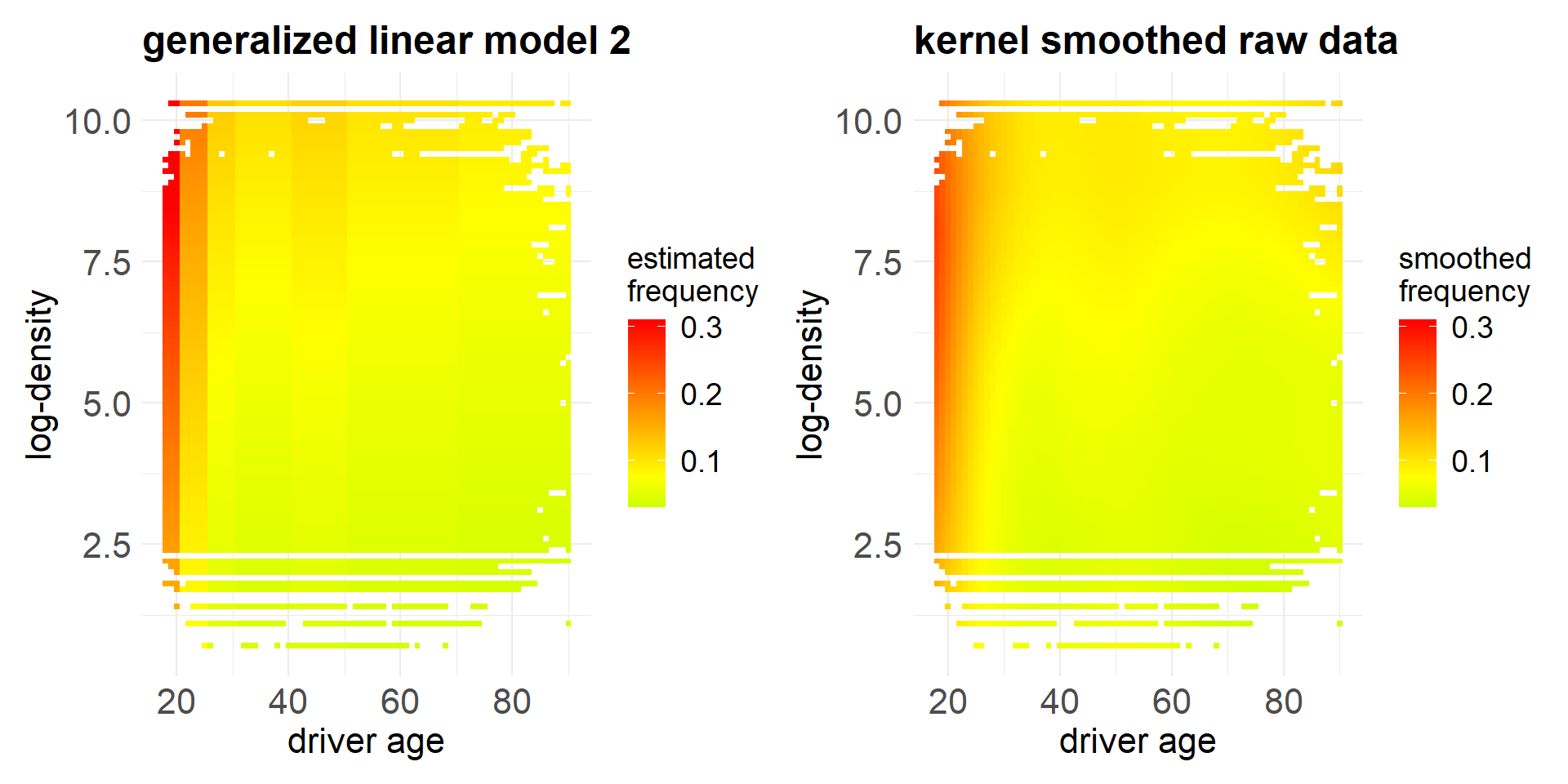
- This second GLM does not (easily) allow for diagonal structure. This is a motivation to consider more advanced regression models.
4 Gradient boosting machine
As a preliminary machine learning regression model, we present a gradient boosting machine (GBM).
GBMs belong to the most powerful techniques on tabular data.
A GBM partitions the covariate space into different (homogeneous) subsets and it estimates the frequency on each subset.
We only present the resulting heatmap on the two selected covariates, and for technical details we refer to the GBM notebook.
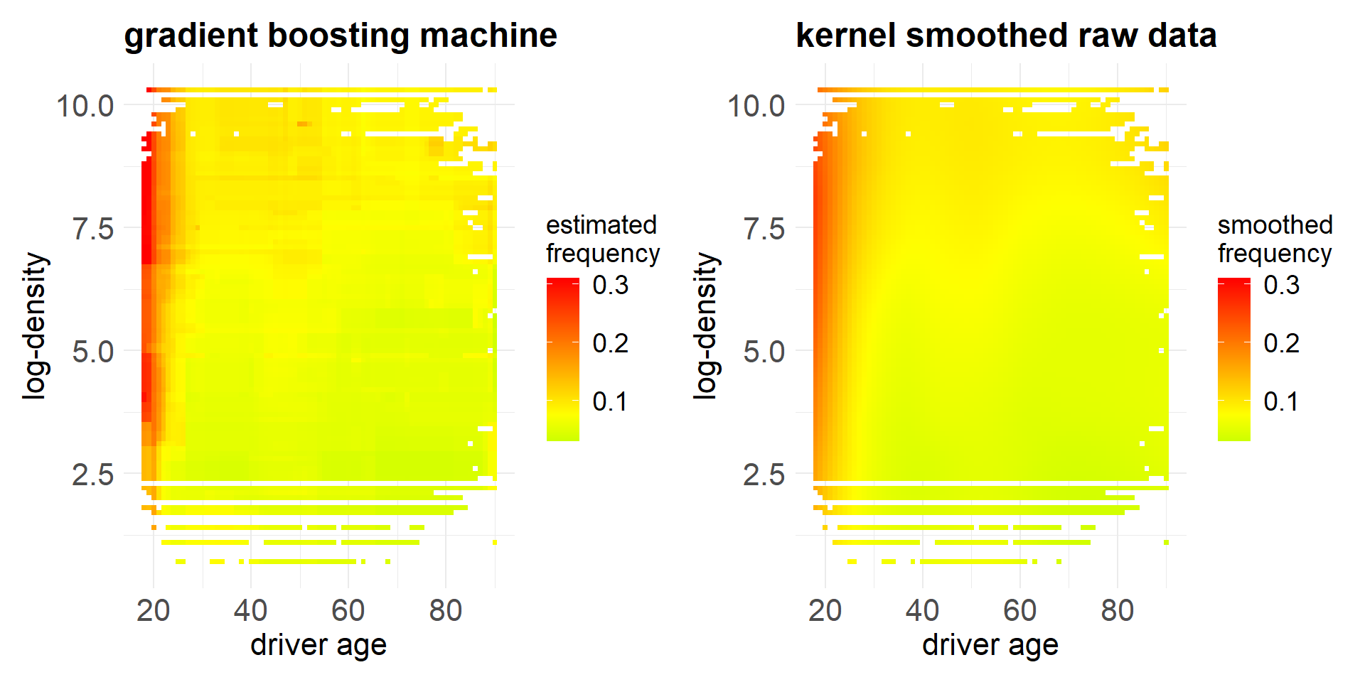
We observe that the GBM reflects the observed (smoothed) data very well.
The only criticism that one may have is that the resulting regression function is not smooth and that it cannot easily be extrapolated.
A crucial question that one may have is whether this GBM only extracts the structural (systematic) part or whether it also reflects some of the noise in the observed data. This would not be good, because the noisy part is not structure that will replicate in the future.
This question of in-sample over-fitting is recurrent to all statistical and machine learning methods, and it will be discussed in detail below.
We are now ready to take off this process of statistical modeling and machine learning.
Copyright
© The Authors
This notebook and these slides are part of the project “AI Tools for Actuaries”. The lecture notes can be downloaded from:
https://papers.ssrn.com/sol3/papers.cfm?abstract_id=5162304
\(\,\)
- This material is provided to reusers to distribute, remix, adapt, and build upon the material in any medium or format for noncommercial purposes only, and only so long as attribution and credit is given to the original authors and source, and if you indicate if changes were made. This aligns with the Creative Commons Attribution 4.0 International License CC BY-NC.
References
Dutang, C., Charpentier, A. and Gallic, E. (2024) “Insurance dataset.” Available at: https://dutangc.github.io/CASdatasets/.
Wüthrich, M.V. and Merz, M. (2023) Statistical foundations of actuarial learning and its applications. Springer. Available at: https://doi.org/10.1007/978-3-031-12409-9.