Lecture 2: Exponential Dispersion Family &
Generalized Linear Models

Deep Learning for Actuarial Modeling
36th International Summer School SAA
University of Lausanne

Author

Ronald Richman, Salvatore Scognamiglio, Mario V. Wüthrich

Published

September 8, 2025

Abstract

First, this lecture gives an introduction to the exponential dispersion family (EDF), which is the main family of distributions considered for regression modeling. Second, it introduces the framework of generalized linear models (GLMs).

1 Introduction

Overview

This lecture introduces the exponential dispersion family (EDF). The EDF is the most important family of distributions for regression modeling. Within this family, maximum likelihood estimation (MLE) is equivalent to deviance loss minimization. Therefore, this probabilistic framework gives us a foundation to select the objective function for model fitting.

This theoretical framework is then applied to the class of generalized linear models (GLMs). GLMs are the core regression models and they form the technical basis for more advanced regression tools like neural networks. In particular, in the next lecture, we are going to present neural networks as an extension of GLMs.

This lecture covers Chapters 1-3 of Wüthrich et al. (2025).

Desirable properties of actuarial regression models

Desirable characteristics of predictive models in insurance:
1. provide accurate forecasts;
2. smoothness properties so that forecasts do not drastically change, if one slightly perturbs the inputs;
3. sparsity and simplicity; one aims for a parsimonious model;
4. inner functioning of the model should be intuitive and explainable;
5. good finite sample properties and credible parameter estimates;
6. quantifiable prediction uncertainty;
7. (manually) adaptable to expert knowledge;
8. compliant with regulation, and one should be able to verify this.
Typically, one needs to compromise among these requirements.

2 Exponential dispersion family

A random variable \(Y \sim {\rm EDF}(\theta, \varphi/v; \kappa)\) belongs to the EDF if it has a density of the form \[ Y ~\sim~ f_\theta(y) = \exp\left(\frac{y\theta-\kappa(\theta)}{\varphi/v}+c(y, \varphi/v)\right),\] with

canonical parameter \(\theta \in \boldsymbol{\Theta}\subseteq {\mathbb R}\),
cumulant function \(\kappa : \boldsymbol{\Theta} \to {\mathbb R}\),
dispersion parameter \(\varphi>0\),
weight/volume/exposure \(v>0\);
the meaning of the remaining terms is less relevant for our purposes.

2.1 Exponential dispersion family: main takeaways

The EDF definition looks a bit complicated, but there are only the following points that we need to take from this definition.

The cumulant function \(\kappa\) fully determines the specific type of distribution of \(Y\): it includes, e.g., the Poisson, gamma and Tweedie’s class.
The canonical parameter \(\theta\) is the model parameter to be estimated; the regression structure will enter this canonical parameter.
The mean is given by \[ {\mathbb E}\left[ Y\right]=\kappa'(\theta).\]
The variance is given by \[ {\rm Var}\left( Y\right)=\frac{\varphi}{v}\kappa''(\theta) %=\frac{\varphi}{v}\kappa''\left((\kappa')^{-1}(\mu_0)\right) .\]

Inverse function \(h:=(\kappa')^{-1}\) is the canonical link of the chosen EDF.
The canonical link \(h\) allows one to identify the mean and the canonical parameter of the selected EDF by \[ {\mathbb E}\left[ Y\right]=\kappa'(\theta)\quad\Longleftrightarrow\quad h\left({\mathbb E}\left[ Y\right]\right)=\theta.\]
This is one-to-one relationship between the mean and the canonical parameter, and we can use either of them for model fitting.
The EDF model class is fitted with MLE.

Model fitting

MLE within the EDF is equivalent to deviance loss minimization.

2.2 Deviance loss function

Select \(Y \sim {\rm EDF}(\theta, \varphi/v; \kappa)\) with cumulant function \(\kappa\).
The deviance loss function of the selected EDF is given by \[ L(y,m) = 2\, \frac{\varphi}{v}\left( \log \left(f_{h(y)}(y)\right) - \log \left(f_{h(m)}(y)\right)\right) \ge 0,\] for observation \(y\) and mean \(m\).
Deviance losses are strictly consistent for mean estimation: this is a necessary condition for appropriate model fitting; Gneiting (2011).
If the selected deviance loss meets the properties of the responses \(Y\), in particular, if it has the same variance behavior, the estimation procedure is optimal in the sense of best asymptotic normal; Gourieroux, Monfort and Trognon (1984).

Finite sample estimation

Always select the deviance loss that aligns with the EDF properties of \(Y\) for model fitting (i.e., select the correct \(\kappa\) for \(Y\)).

Some examples:

EDF distribution	cumulant \(\kappa(\theta)\)	deviance loss \(L(y,m)\)
Gaussian	\(\theta^2/2\)	\((y-m)^2\)
gamma	\(-\log(-\theta)\)	\(2\left((y-m)/m+\log(m/y)\right)\)
inverse Gaussian	\(-\sqrt{-2\theta}\)	\((y-m)^2/(m^2y)\)
Poisson	\(e^\theta\)	\(2\left(m-y-y\log(m/y)\right)\)
Tweedie \(p\in (1,2)\)	\(\frac{((1-p)\theta)^{\frac{2-p}{1-p}}}{2-p}\)	\(2\left(y\frac{y^{1-p}-m^{1-p}}{1-p}-\frac{y^{2-p}-m^{2-p}}{2-p}\right)\)
Bernoulli	\(\log(1+e^\theta)\)	\(2\left(-y \log (m) - (1-y)\log(1-m)\right)\)

3 Model validation and model selection

Select a deviance loss \(L(y,m)\) for model fitting.
Based on a learning sample \({\cal L}=(Y_i, \boldsymbol{X}_i, v_i)_{i=1}^n\), one minimizes the in-sample loss \[ \widehat{\mu}_{\cal L} ~\in~ \underset{ \mu}{\arg\min}\, \sum_{i=1}^n \frac{v_i}{\varphi}\, L\left(Y_i,\mu(\boldsymbol{X}_i)\right);\] a lower index is added to \(\widehat{\mu}_{\cal L}\) to highlight that this step is performed on the learning sample \({\cal L}\).
Model validation and model selection should not be done on the (same) learning sample \({\cal L}\). This would give a too optimistic judgement: a more complex model always has a smaller loss than a nested simpler model.

Model validation needs to be done on an independent test sample (hold-out sample) \({\cal T}=(Y_t, \boldsymbol{X}_t, v_t)_{t=1}^m\).
\(\textcolor{blue}{\cal L}\) and \(\textcolor{red}{\cal T}\) should be independent and contain i.i.d. data following the same law as \((Y, \boldsymbol{X}, v)\).
The out-of-sample loss (generalization loss) is defined by \[ \widehat{\rm GL}(\textcolor{red}{\cal T}, \widehat{\mu}_{\textcolor{blue}{\cal L}})= \frac{1}{\sum_{{\textcolor{red}{t=1}}}^{\textcolor{red}{m}} v_{\textcolor{red}{t}}/\varphi}\,\sum_{{\textcolor{red}{t=1}}}^{\textcolor{red}{m}} \frac{v_{\textcolor{red}{t}}}{\varphi}\, L\left(Y_{\textcolor{red}{t}},\widehat{\mu}_{\textcolor{blue}{\cal L}}(\boldsymbol{X}_{\textcolor{red}{t}})\right).\]
This out-of-sample loss is the main workhorse for model validation and model selection in machine learning and AI.

4 GLM regression function

Consider \(q\)-dimensional real-valued covariates \(\boldsymbol{X}=(X_1,\ldots, X_q)^\top\).
Select a smooth and strictly increasing link function \(g\).
A GLM regression function is given by \[ \boldsymbol{X}~\mapsto~g(\mu_{\vartheta}(\boldsymbol{X})) = \vartheta_0 + \sum_{j=1}^q \vartheta_j X_j=: \left\langle \vartheta, \boldsymbol{X} \right\rangle,\] with GLM parameter \(\vartheta=(\vartheta_0,\ldots, \vartheta_q)^\top \in {\mathbb R}^{q+1}\).
This implies conditional mean for response \(Y\), given covariates \(\boldsymbol{X}\), \[ \mu_{\vartheta}(\boldsymbol{X}) = {\mathbb E} \left[\left. Y \right|\boldsymbol{X}\right] =g^{-1} \left\langle \vartheta, \boldsymbol{X} \right\rangle.\]
There is a linear structure in \(\boldsymbol{X}\) up to the link transformation \(g^{-1}\).

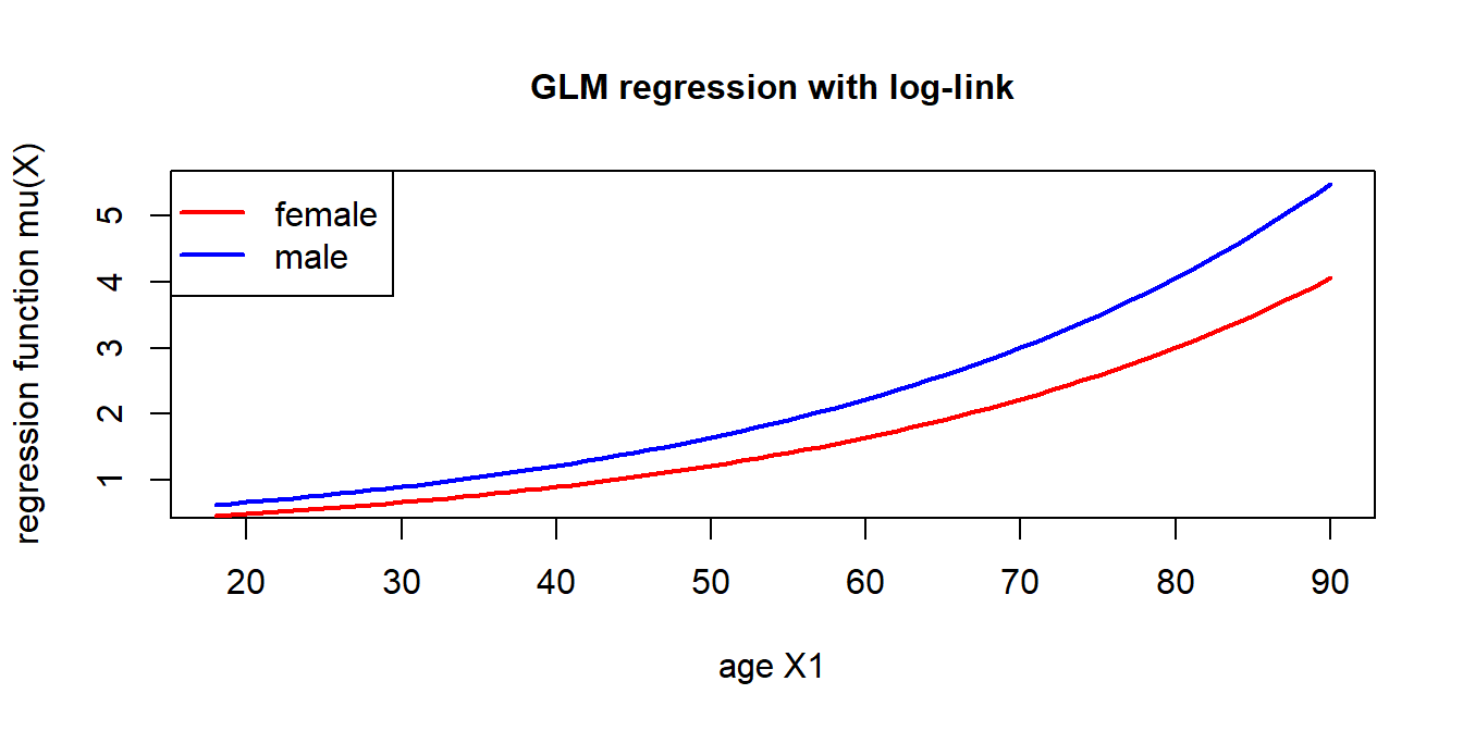
4.1 Log-link example

The log-link is by far the most popular link for actuarial modeling (under positive claims \(Y\)) \[g(\cdot)=\log(\cdot).\]
This implies a multiplicative (price) mean functional \[ \boldsymbol{X}~\mapsto~ \mu_{\vartheta}(\boldsymbol{X}) = {\mathbb E} \left[\left. Y \right|\boldsymbol{X}\right] =\exp \left\langle \vartheta, \boldsymbol{X} \right\rangle = e^{\vartheta_0} \prod_{j=1}^q e^{\vartheta_j X_j}.\]
The price relativities \(e^{\vartheta_j X_j}\) are easily interpretable.
The bias parameter \(\vartheta_0 \in {\mathbb R}\) is used to calibrate the overall level.

The graph shows: \(q=2\) with \(X_1 \in [18,90]\) being the age and \(X_2\in \{0,1\}=\{{\rm male}, {\rm female}\}\) the gender of the policyholder.

This example has regression parameter components \(\vartheta_1>0\) and \(\vartheta_2<0\).

4.2 EDF and the canonical link

Starting from \(Y \sim {\rm EDF}(\theta, \varphi/v; \kappa)\), there is the special link choice \[ g(\cdot)=h(\cdot)=(\kappa')^{-1}(\cdot).\]
This link is called the canonical link of the selected EDF.
Under the canonical link choice, there is the identity \[ \theta =h \left({\mathbb E} \left[\left. Y \right|\boldsymbol{X}\right]\right)= \langle \vartheta, \boldsymbol{X} \rangle.\]
That is, under the canonical link choice, the canonical parameter \(\theta\) receives the linear structure \(\langle \vartheta, \boldsymbol{X} \rangle\); called linear predictor.
Remark: \(\theta\) denotes the canonical parameter and \(\vartheta\) the regression parameter.

Canonical links have good mathematical properties, e.g.,
1. the MLE of a GLM is unique;
2. the resulting fitted GLM fulfills the balance property.
Generally, the support of \(\theta\) is not necessarily the entire real line \({\mathbb R}\). This may lead to domain constraints which are difficult to meet in numerical applications under the canonical link choice.
Therefore, under positive responses \(Y\), e.g., in the gamma EDF case, the log-link is preferred over the canonical link.
The log-link is the canonical link (if and only if) of the Poisson model.

EDF distribution	canonical link \(h(\mu)\)	support of \(\theta\)	mean parameter space
Gaussian	\(\mu\)	\({\mathbb R}\)	\({\mathbb R}\)
gamma	\(-1/\mu\)	\((-\infty, 0)\)	\((0,\infty)\)
inverse Gaussian	\(-1/(2\mu^2)\)	\((-\infty,0]\)	\((0,\infty)\)
Poisson	\(\log(\mu)\)	\({\mathbb R}\)	\((0,\infty)\)
Tweedie	\(\mu^{1-p}/(1-p)\)	\((-\infty, 0)\)	\((0,\infty)\)
Bernoulli	\(\log(\mu/(1-\mu))\)	\({\mathbb R}\)	\((0,1)\)

In the Gaussian (identity link), the Poisson (log-link) and the Bernoulli (logit link) cases one typically selects the canonical link.
In the other cases one selects the log-link.

5 GLM fitting and examples

Construct the log-likelihood function of the learning sample \({\cal L}=(Y_i,\boldsymbol{X}_i,v_i)_{i=1}^n\) assuming independent EDF instances \[ \vartheta ~\mapsto ~ \ell(\vartheta)=\sum_{i=1}^n \frac{v_i}{\varphi} \left[Y_i \,h\left(\mu_{\vartheta}(\boldsymbol{X}_i)\right) -\kappa\left(h\left(\mu_{\vartheta}(\boldsymbol{X}_i)\right)\right)\right]+c(Y_i, \varphi/v_i).\]
The MLE is found by solving, subject to existence, \[ \widehat{\vartheta}^{\rm MLE} ~ \in ~ \underset{\vartheta}{\arg\max}~\ell(\vartheta).\]
This is solved numerically by Fisher’s scoring method or the IRLS algorithm; see Nelder and Wedderburn (1972).
This looks complicated, but actually it’s not: consider deviance losses!

5.1 Relationship to deviance losses

The deviance loss \(L\) of any EDF density \(f_\theta\) with cumulant function \(\kappa\) gives a strictly consistent loss for mean estimation \[ L(y,m) = 2\frac{\varphi}{v}\left[ \log \left(f_{h(y)}(y)\right) - \log \left(f_{h(m)}(y)\right)\right]\ge 0.\]
Instead of maximizing the log-likelihood of the chosen EDF, one can equally minimize this deviance loss to get the same result.
This deviance loss minimization looks nicer \[\widehat{\vartheta}^{\rm MLE} ~ \in ~ \underset{\vartheta}{\arg\min}~ \sum_{i=1}^n \frac{v_i}{\varphi}\, L(Y_i, \mu_{\vartheta}(\boldsymbol{X}_i)).\]
Recall: The correct deviance loss function \(L\) (w.r.t. \(Y\)) has the best finite sample properties; Gourieroux, Monfort and Trognon (1984).

5.2 Example: Poisson log-link GLM

Assume \(Y_i\) are Poisson; this is EDF with \(\kappa(\cdot)=\exp(\cdot)\).
Select a log-link GLM regression function with parameter \(\vartheta \in {\mathbb R}^{q+1}\) \[ \boldsymbol{X}~\mapsto~ \log(\mu_{\vartheta}(\boldsymbol{X})) = \vartheta_0 +\sum_{j=1}^q \vartheta_j X_j.\]
The Poisson deviance loss minimization solves \[ \widehat{\vartheta}^{\rm MLE} = \underset{\vartheta \in {\mathbb R}^{q+1}}{\arg\min}~\sum_{i=1}^n 2v_i\left(\mu_{\vartheta}(\boldsymbol{X}_i)-Y_i-Y_i\,\log\left(\frac{\mu_{\vartheta}(\boldsymbol{X}_i)}{Y_i}\right)\right).\]
\(v_i>0\) are the time exposures, and \(Y_i=N_i/v_i\) are the claims frequencies for the observed claim counts \(N_i \in {\mathbb N}_0\).
The dispersion in the Poisson model is \(\varphi=1\).

5.3 GLM example: French MTPL data

We revisit the French MTPL claims count data from the previous lecture.

load(file="../Data/freMTPL2freqClean.rda")
dat <- freMTPL2freqClean
str(dat)

The (cleaned) data is illustrated below.
The last line shows whether the instance belongs to the learning sample ‘L’ or the test sample ‘T’; this is the identical (random) learning-test set partition as in Wüthrich and Merz (2023) (also the randomized order is identical which will be important in stochastic gradient descent fitting of networks).
The variable type ‘Factor’ denotes categorical covariates. In the subsequent GLM implementation, they will automatically (internally) be encoded by dummy coding (described in a later lecture).

'data.frame':   678007 obs. of  14 variables:
 $ IDpol     : num  4156370 4006798 6084964 2228865 4141911 ...
 $ Exposure  : num  0.06 0.29 0.46 0.08 1 0.6 0.08 0.12 1 0.12 ...
 $ Area      : Factor w/ 6 levels "A","B","C","D",..: 4 5 3 4 1 3 3 4 2 5 ...
 $ VehPower  : int  6 6 7 4 5 5 4 4 5 5 ...
 $ VehAge    : int  6 7 10 15 22 2 15 2 4 6 ...
 $ DrivAge   : int  20 29 27 34 44 25 29 50 29 54 ...
 $ BonusMalus: int  100 59 68 50 50 90 85 50 72 103 ...
 $ VehBrand  : Factor w/ 11 levels "B1","B2","B3",..: 2 9 1 2 3 5 2 9 3 1 ...
 $ VehGas    : Factor w/ 2 levels "Diesel","Regular": 2 1 1 2 1 2 2 2 1 2 ...
 $ Density   : int  525 2498 123 1109 34 129 196 629 66 3744 ...
 $ Region    : Factor w/ 22 levels "R11","R21","R22",..: 18 15 18 5 15 9 18 2 15 21 ...
 $ ClaimTotal: num  0 0 0 0 0 0 0 0 0 0 ...
 $ ClaimNb   : num  0 0 0 0 0 0 0 0 0 0 ...
 $ LearnTest : chr  "L" "L" "L" "L" ...

Pre-process data for GLM (this is the feature-engineering step):

dat$AreaGLM       <- as.integer(dat$Area)
dat$VehPowerGLM   <- as.factor(pmin(dat$VehPower, 9))
dat$VehAgeGLM     <- as.factor(cut(dat$VehAge, c(0,5,12,101), 
                       labels = c("0-5", "6-12", "12+"),
                       include.lowest = TRUE))
dat$DrivAgeGLM    <- as.factor(cut(dat$DrivAge, c(18,20,25,30,40,50,70,101), 
                       labels = c("18-20", "21-25", "26-30", "31-40", "41-50", "51-70", "71+"),
                       include.lowest = TRUE))
dat$DrivAgeGLM    <- relevel(dat[,"DrivAgeGLM"], ref="31-40")
dat$BonusMalusGLM <- pmin(dat$BonusMalus, 150)  
dat$DensityGLM    <- log(dat$Density)  
#
learn <- dat[which(dat$LearnTest=='L'),]
test  <- dat[which(dat$LearnTest=='T'),]

Fit/learn a Poisson log-link GLM (with time exposures):

d.glm <- glm(ClaimNb ~ DrivAgeGLM + VehBrand + VehGas + DensityGLM + AreaGLM, data=learn, offset=log(Exposure), family=poisson())
summary(d.glm)

...
Coefficients:
                 Estimate Std. Error z value Pr(>|z|)    
(Intercept)     -3.258957   0.034102 -95.564  < 2e-16 ***
DrivAgeGLM18-20  1.275057   0.044964  28.358  < 2e-16 ***
DrivAgeGLM21-25  0.641668   0.028659  22.390  < 2e-16 ***
DrivAgeGLM26-30  0.153978   0.025703   5.991 2.09e-09 ***
DrivAgeGLM41-50  0.121999   0.018925   6.447 1.14e-10 ***
DrivAgeGLM51-70 -0.017036   0.018525  -0.920 0.357776    
DrivAgeGLM71+   -0.047132   0.029964  -1.573 0.115726    
VehBrandB2       0.007238   0.018084   0.400 0.688958    
...

...
VehBrandB3       0.085213   0.025049   3.402 0.000669 ***
VehBrandB4       0.034577   0.034523   1.002 0.316553    
VehBrandB5       0.122826   0.028792   4.266 1.99e-05 ***
VehBrandB6       0.080310   0.032325   2.484 0.012976 *  
VehBrandB10      0.067790   0.040607   1.669 0.095032 .  
VehBrandB11      0.221375   0.043348   5.107 3.27e-07 ***
VehBrandB12     -0.152185   0.020866  -7.294 3.02e-13 ***
VehBrandB13      0.101940   0.047062   2.166 0.030306 *  
VehBrandB14     -0.201833   0.093754  -2.153 0.031336 *  
VehGasRegular   -0.198766   0.013323 -14.920  < 2e-16 ***
DensityGLM       0.094453   0.014623   6.459 1.05e-10 ***
AreaGLM          0.028487   0.019909   1.431 0.152471    
---
Signif. codes:  0 '***' 0.001 '**' 0.01 '*' 0.05 '.' 0.1 ' ' 1

(Dispersion parameter for poisson family taken to be 1)
...

...

    Null deviance: 153852  on 610205  degrees of freedom
Residual deviance: 151375  on 610186  degrees of freedom
AIC: 197067

Number of Fisher Scoring iterations: 6
...

\(\,\)

For better visibility and faster computation, we did not include all available covariates. For benchmarking, later on an optimal GLM will be selected.

5.4 Poisson deviance loss: in-sample and out-of-sample

For model fitting and model selection: study the in-sample and the out-of-sample Poisson deviance losses on the learning sample \({\cal L}=(Y_i,\boldsymbol{X}_i,v_i)_{i=1}^n\) and the test sample \({\cal T}=(Y_t,\boldsymbol{X}_t,v_t)_{t=1}^m\), respectively.
The scaled in-sample Poisson deviance loss on \({\cal L}\) is given by \[ \frac{1}{\sum_{i=1}^n v_i} \sum_{i=1}^n 2 v_i\left( \mu_{\widehat{\vartheta}^{\rm MLE}}(\boldsymbol{X}_i)-Y_i-Y_i \log \left(\frac{\mu_{\widehat{\vartheta}^{\rm MLE}}(\boldsymbol{X}_i)}{Y_i}\right)\right).\]
The scaled out-of-sample Poisson deviance loss on \({\cal T}\) is given by \[ \frac{1}{\sum_{t=1}^m v_t} \sum_{t=1}^m 2 v_t\left( \mu_{\widehat{\vartheta}^{\rm MLE}}(\boldsymbol{X}_t)-Y_t-Y_t \log \left(\frac{\mu_{\widehat{\vartheta}^{\rm MLE}}(\boldsymbol{X}_t)}{Y_t}\right)\right).\]

Poisson.Deviance <- function(pred, obs, weights){  
  100*2*(sum(pred)-sum(obs)+sum(log((obs/pred)^(obs))))/sum(weights)} 
# 
learn$GLM <- fitted(d.glm)
test$GLM  <- predict(d.glm, newdata=test, type="response")
#
# Poisson deviances are generally scaled with 100 for better visibility
round(c(Poisson.Deviance(learn$GLM, learn$ClaimNb, learn$Exposure), Poisson.Deviance(test$GLM, test$ClaimNb, test$Exposure)), 3)

[1] 46.954 47.179

round(100*d.glm$deviance/sum(learn$Exposure),3)   # check with GLM output

[1] 46.954

These figures are in \(10^{-2}\) units (throughout this lecture).
This GLM can be improved because we did not consider all covariates.

5.5 Offsets vs. weights

The above code does not consider claims frequencies \(Y_i=N_i/v_i\), but rather claims counts \(N_i \in \mathbb{N}_0\).
Thus, we have fitted a GLM to \[ \mathbb{E}[N_i|\boldsymbol{X}_i] =v_i\,\mathbb{E}[Y_i|\boldsymbol{X}_i] =v_i\,\exp \left\langle \vartheta, \boldsymbol{X}_i \right\rangle =\exp \left(\left\langle \vartheta, \boldsymbol{X}_i \right\rangle + \log v_i \right).\]
This uses \(\log v_i\) as an offset (not involving a regression parameter) and regresses \[N_i \sim \boldsymbol{X}_i + {\rm offset}(\log v_i),\] with weights equal to 1; see code above.
The EDF-GLM framework proposes to regress \(Y_i \sim \boldsymbol{X}_i\) with weights \(v_i\).
For the log-link Poisson regression the two approaches are equivalent.
We verify this by revisiting the above Poisson GLM example.

# fitting claims frequencies Y=N/v with weights v
d.glm.weights <- glm(ClaimNb/Exposure ~ DrivAgeGLM + VehBrand + VehGas + DensityGLM + AreaGLM, data=learn, weights=Exposure, family=quasipoisson())

# for predicting the counts we need to rescale with the weights  
learn$GLM.W <- fitted(d.glm.weights)*learn$Exposure
test$GLM.W  <- predict(d.glm.weights, newdata=test, type="response")*test$Exposure
#
round(c(Poisson.Deviance(learn$GLM.W, learn$ClaimNb, learn$Exposure), Poisson.Deviance(test$GLM.W, test$ClaimNb, test$Exposure)), 3)

[1] 46.954 47.179

This in-sample and out-of-sample losses are identical to above.

Takeaways and outlook

The GLM regression function is the base case that will be extended to neural network regression functions.
GLM regression function: \[ \boldsymbol{X}~\mapsto~g(\mu_{\vartheta}(\boldsymbol{X})) = \vartheta_0 + \sum_{j=1}^q \vartheta_j X_j= \left\langle \vartheta, \boldsymbol{X} \right\rangle.\]
Neural network regression function: \[\begin{eqnarray*} \boldsymbol{X}~\mapsto~g(\mu_{\vartheta}(\boldsymbol{X})) &=& w^{(d+1)}_0 + \sum_{j=1}^{q_d} w^{(d+1)}_j \textcolor{blue}{z_j^{(d:1)}}(\boldsymbol{X}) \\&=& \left\langle \boldsymbol{w}^{(d+1)}, \textcolor{blue}{\boldsymbol{z}^{(d:1)}}(\boldsymbol{X}) \right\rangle, \end{eqnarray*}\] with a deep neural network (feature extractor) \(\textcolor{blue}{\boldsymbol{z}^{(d:1)}}:{\mathbb R}^{q}\to {\mathbb R}^{q_d}\).

Copyright

© The Authors
This notebook and these slides are part of the project “AI Tools for Actuaries”. The lecture notes can be downloaded from:

https://papers.ssrn.com/sol3/papers.cfm?abstract_id=5162304

\(\,\)

This material is provided to reusers to distribute, remix, adapt, and build upon the material in any medium or format for noncommercial purposes only, and only so long as attribution and credit is given to the original authors and source, and if you indicate if changes were made. This aligns with the Creative Commons Attribution 4.0 International License CC BY-NC.

References

Gneiting, T. (2011) “Making and evaluating point forecasts,” Journal of the American Statistical Association, 106(494), pp. 746–762. Available at: https://doi.org/10.1198/jasa.2011.r10138.

Gourieroux, C., Monfort, A. and Trognon, A. (1984) “Pseudo maximum likelihood methods: theory,” Econometrica, 52(3), pp. 681–700. Available at: https://www.jstor.org/stable/1913471?seq=1.

Nelder, J.A. and Wedderburn, R.W.M. (1972) “Generalized linear models,” Journal of the Royal Statistical Society. Series A (General), 135(3), pp. 370–384. Available at: https://doi.org/10.2307/2344614.

Wüthrich, M.V. et al. (2025) “AI Tools for Actuaries,” SSRN Manuscript [Preprint]. Available at: https://papers.ssrn.com/sol3/papers.cfm?abstract_id=5162304.

Wüthrich, M.V. and Merz, M. (2023) Statistical foundations of actuarial learning and its applications. Springer. Available at: https://doi.org/10.1007/978-3-031-12409-9.