FNN.embed <- function(seed, qq, kk, bb){
k_clear_session()
set.seed(seed)
set_random_seed(seed)
Design <- layer_input(shape = c(qq[1]), dtype = 'float32')
Volume <- layer_input(shape = c(1), dtype = 'float32')
#
# define the entity embeddings (levels are encoded by integers)
BrandEmb = Design[,qq[1]-1] %>%
layer_embedding(input_dim = kk[1], output_dim = bb[1], input_length = 1) %>% layer_flatten()
#
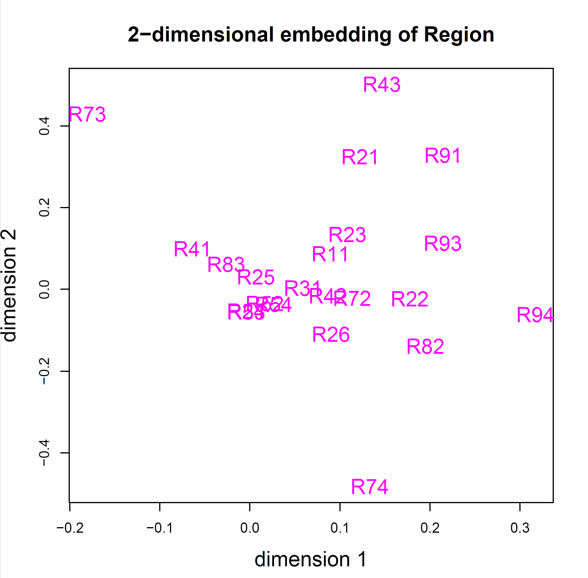
RegionEmb = Design[,qq[1]] %>%
layer_embedding(input_dim = kk[2], output_dim = bb[2], input_length = 1) %>% layer_flatten()Lecture 6: Covariate Engineering & Entity Embedding
Deep Learning for Actuarial Modeling
36th International Summer School SAA
University of Lausanne
36th International Summer School SAA
University of Lausanne
Abstract
An important part of regression modeling is covariate engineering. This involves dealing with categorical covariates, but it also deals with bringing continuous covariates into a suitable form.
1 Introduction
This lecture covers Chapter 4 of Wüthrich et al. (2025).
2 Categorical covariates
Categorical covariates (nominal or ordinal) need pre-processing to bring them into a numerical form. This is done by entity embedding.
Consider a categorical covariate \(X\) taking values in a finite set \({\cal A}=\{a_1, \ldots, a_K \}\) having \(K\) different levels.
The running example in this lecture has \(K=6\) levels: \[\begin{eqnarray*} {\cal A} &=& \Big\{\,\text{accountant}, \text{ actuary}, \text{ economist}, \\&&\hspace{8ex} \text{\qquad\qquad quant}, \text{ statistician}, \text{ underwriter}\Big\}. \end{eqnarray*}\]
We need to bring this into a numerical form for regression modeling.
2.1 Ordinal categorical covariates
For ordinal (ordered) levels \((a_k)_{k=1}^K\), use a 1-dimensional entity embedding \[ X \in {\cal A} ~\mapsto ~\sum\nolimits_{k=1}^K k \, \mathbf{1}_{\{X=a_k\}} \in {\mathbb R}.\]
Our running example has an alphabetical ordering.
| level | embedding |
|---|---|
| accountant | 1 |
| actuary | 2 |
| economist | 3 |
| quant | 4 |
| statistician | 5 |
| underwriter | 6 |
One may argue that the alphabetical order is risk insensitive (not useful).
2.2 One-hot encoding
One-hot encoding maps each level \(a_k\) to a basis vector in \({\mathbb R}^K\) \[ X \in {\cal A} ~\mapsto ~ \left(\mathbf{1}_{\{X=a_1\}}, \ldots, \mathbf{1}_{\{X=a_K\}}\right)^\top \in {\mathbb R}^K.\]
| level | ||||||
|---|---|---|---|---|---|---|
| accountant | 1 | 0 | 0 | 0 | 0 | 0 |
| actuary | 0 | 1 | 0 | 0 | 0 | 0 |
| economist | 0 | 0 | 1 | 0 | 0 | 0 |
| quant | 0 | 0 | 0 | 1 | 0 | 0 |
| statistician | 0 | 0 | 0 | 0 | 1 | 0 |
| underwriter | 0 | 0 | 0 | 0 | 0 | 1 |
One-hot encoding does not lead to full rank encodings because there is a redundancy (the first \(K-1\) components are sufficient).
2.3 Dummy coding
Dummy coding selects a reference level, e.g., \(a_2=\text{actuary}\). Based on this selection, all other levels are measured relative to this reference level \[ X \in {\cal A} ~\mapsto ~ \left(\mathbf{1}_{\{X=a_1\}}, \mathbf{1}_{\{X=a_3\}}, \mathbf{1}_{\{x=a_4\}},\ldots, \mathbf{1}_{\{X=a_K\}}\right)^\top \in {\mathbb R}^{K-1}. \]
| level | |||||
|---|---|---|---|---|---|
| accountant | 1 | 0 | 0 | 0 | 0 |
| actuary | 0 | 0 | 0 | 0 | 0 |
| economist | 0 | 1 | 0 | 0 | 0 |
| quant | 0 | 0 | 1 | 0 | 0 |
| statistician | 0 | 0 | 0 | 1 | 0 |
| underwriter | 0 | 0 | 0 | 0 | 1 |
This leads to full rank, but also to sparsity on large datasets, i.e., most of the entries are zero (for \(K\) large). This may be problematic numerically.
2.4 Entity embedding
Borrowing ideas from natural language processing (NLP), use low dimensional entity embeddings, with proximity related to similarity; see Brébisson et al. (2015), Guo and Berkhahn (2016), Richman (2021).
Choose an embedding dimension \(b \in {\mathbb N}\), this is a hyper-parameter selected by the modeler, typically \(b\ll K\).
An entity embedding (EE) is defined by \[ \boldsymbol{e}^{\rm EE}: {\cal A} \to {\mathbb R}^b, \qquad X \mapsto \boldsymbol{e}^{\rm EE}(X).\]
In total this entity embedding involves \(b\cdot K\) embedding weights.
Embedding weights need to be determined either by the modeler (manually) or during the model fitting procedure (algorithmically), and proximity in embedding should reflect similarity in (risk) behavior.
- Manually chosen example with \(b\cdot K=24\) embedding weights.
| level | finance | maths | stats | liability | |
|---|---|---|---|---|---|
| accountant | 0.5 | 0 | 0 | 0 | |
| actuary | 0.5 | 0.3 | 0.5 | 0.5 | |
| economist | 0.5 | 0.2 | 0.5 | 0 | |
| quant | 0.7 | 0.3 | 0.3 | 0 | |
| statistician | 0 | 0.5 | 0.8 | 0 | |
| underwriter | 0 | 0.1 | 0.1 | 0.8 |
Note: the weights do not need to be normalized, i.e., only proximity in \({\mathbb R}^b\) is relevant.
In neural networks, this can be achieved by setting up a so-called embedding layer. The embedding weights can be learned with stochastic gradient descent.
2.5 Target encoding
Especially for regression trees, one uses target encoding.
Assume a given sample \((Y_i, X_i, v_i)_{i=1}^n\) with categorical covariates \(X_i \in {\cal A}\), real-valued responses \(Y_i\) and weights \(v_i>0\).
Compute the weighted sample means on all levels \(a_k \in {\cal A}\) by \[ \overline{y}_k = \frac{\sum_{i=1}^n v_iY_i\, \mathbf{1}_{\{X_i=a_k\}}} {\sum_{i=1}^n v_i \mathbf{1}_{\{X_i=a_k\}}}.\]
These weighted sample means \((\overline{y}_k)_{k=1}^K\) are used like ordinal levels \[ X \in {\cal A} ~\mapsto ~\sum\nolimits_{k=1}^K \overline{y}_k \, \mathbf{1}_{\{X=a_k\}}.\]
Though convincing initially, this does not consider interactions between covariates, potentially giving misleading results for scarce levels.
2.6 Credibilitized target embedding
For scarce levels, one should credibilitize target encoding; see Micci-Barreca (2001) and Bühlmann (1967).
Problem: Assess how credible the individual estimates \(\overline{y}_k\) are.
Improve unreliable ones by mixing them with the global weighted empirical mean \(\overline{y}=\sum_{i=1}^n v_iY_i/\sum_{i=1}^n v_i\), providing \[ \overline{y}^{\rm cred}_k = \alpha_k\,\overline{y}_k + \left(1-\alpha_k\right) \overline{y},\] with credibility weights for \(1\le k \le K\) \[ \alpha_k = \frac{\sum_{i=1}^n v_i\mathbf{1}_{\{X_i=a_k\}}}{\sum_{i=1}^n v_i\mathbf{1}_{\{X_i=a_k\}}+ \tau}~\in~(0,1].\]
Shrinkage parameter \(\tau \ge 0\) needs to be selected by the modeler.
3 Continuous covariates
In theory, continuous covariates do not need any pre-processing.
In practice, it might be that continuous covariates do not provide the right functional form, or they may live on the wrong scale.
E.g., we may replace a positive covariate \(X>0\) by a 4-dimensional pre-processed covariate \[ X ~\mapsto ~ (X, \log(X), \exp\{X\}, (X-10)^2)^\top.\]
In GLMs, one often discretizes continuous covariates by binning. For a finite partition \((I_k)_{k=1}^K\) of the support of the continuous covariate \(X\), assign categorical labels \(a_k \in {\cal A}\) to \(X\) by setting \[ X ~\mapsto ~ \sum\nolimits_{k=1}^K a_k\, \mathbf{1}_{\{X \in I_k\}}.\]
3.1 Standardization and MinMaxScaler
Gradient descent fitting methods require that all covariate components live on the same scale.
Assume to have \(n\) instances with a continuous covariate \((X_i)_{i=1}^n\).
Standardization considers the transformation \[ X ~\mapsto ~ \frac{X - \widehat{m}}{\widehat{s}},\] with empirical mean \(\widehat{m}\) and empirical standard deviation \(\widehat{s}>0\) of the sample \((X_i)_{i=1}^n\).
The MinMaxScaler is given by the transformation \[ X ~\mapsto ~ 2\,\frac{X - \min_{1\le i \le n}X_i}{\max_{1\le i \le n}X_i-\min_{1\le i \le n}X_i} -1.\]
3.2 Continuous covariate embedding
In recent deep learning architectures, multi-dimensional entity embedding has been beneficial for continuous covariates \(X \in {\mathbb R}\), too.
This allows one to bring continuous covariates to the same \(b\)-dimensional embedding space as the entity embedded categorical covariates.
Select a deep FNN \(\boldsymbol{z}^{(d:1)}: {\mathbb R} \to {\mathbb R}^b\) giving the entity embedding \[ X~\mapsto \boldsymbol{z}^{(d:1)} (X) \in {\mathbb R}^b.\]
We apply this entity embedding to a covariate vector \[\boldsymbol{X}=(X_1, \ldots, X_{q_c}, X_{q_c+1}, \ldots, X_q)^\top,\] with \(q_c\) categorical covariates and \(q-q_c\) continuous covariates.
Applying entity embedding to both the continuous covariates and the categorical covariates with the same embedding dimension \(b\), gives us an input tensor \[ \bigg[\boldsymbol{e}_{1}^{\rm EE}(X_{1}), \ldots, \boldsymbol{e}_{q_c}^{\rm EE}(X_{q_c}), \boldsymbol{z}_{q_c+1}^{(d:1)} (X_{q_c+1}), \ldots, \boldsymbol{z}_{q}^{(d:1)} (X_{q}) \bigg] ~\in ~{\mathbb R}^{b \times q}.\]
The input data \(\boldsymbol{X}\) is now in a tensor structure, suitable to enter attention layers and the Transformer archicecture of Vaswani et al. (2017); see also Richman, Scognamiglio and Wüthrich (2025).
4 Example: French MTPL data
#
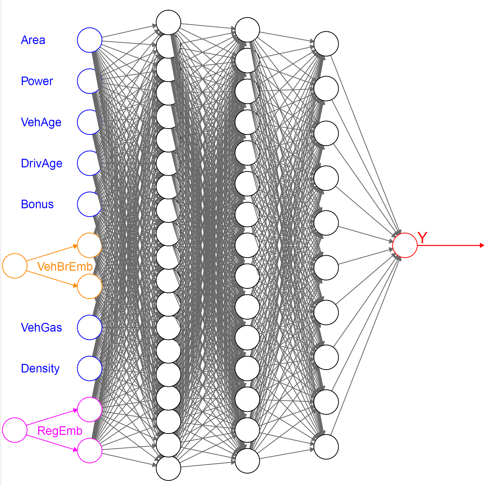
# concatenate entity embeddings and remaining covariates for the FNN
Network = list(Design[,1:(qq[1]-2)], BrandEmb, RegionEmb) %>%
layer_concatenate() %>%
layer_dense(units=qq[2], activation='tanh') %>%
layer_dense(units=qq[3], activation='tanh') %>%
layer_dense(units=qq[4], activation='tanh') %>%
layer_dense(units=1, activation='exponential')
#
Response = list(Network, Volume) %>% layer_multiply()
#
keras_model(inputs = c(Design, Volume), outputs = c(Response))
}Levels are encoded by integers, and after embedding into \({\mathbb R}^b\), they are concatenated with the (standardized) continuous covariates before entering the feature extractor.
...
________________________________________________________________________________
 Layer (type)           Output Shape            Param   Connected to
================================================================================
 embedding (Embedding)  (None, 2)               22      ['tf.__operators__.getit
 embedding_1 (Embeddin  (None, 2)               44      ['tf.__operators__.getit
                                                         'flatten_1[0][0]']
 dense_3 (Dense)        (None, 20)              240     ['concatenate[0][0]']
 dense_2 (Dense)        (None, 15)              315     ['dense_3[0][0]']
 dense_1 (Dense)        (None, 10)              160     ['dense_2[0][0]']
 dense (Dense)          (None, 1)               11      ['dense_1[0][0]']
                                                         'input_2[0][0]']
================================================================================
Total params: 792 (3.09 KB)
Trainable params: 792 (3.09 KB)
Non-trainable params: 0 (0.00 Byte)
...
Results
| model | in-sample loss | out-of-sample loss | balance (in %) |
|---|---|---|---|
| Poisson null model | 47.722 | 47.967 | 7.36 |
| Poisson GLM | 45.585 | 45.435 | 7.36 |
| Poisson FNN | 44.846 | 44.925 | 7.17 |
| nagging predictor | 44.849 | 44.874 | 7.36 |
| embedding FNN | 45.030 | 44.948 | 7.16 |
| embed nagging predictor | 44.636 | 44.864 | 7.36 |
For the nagging predictor we use \(M=10\) individual network fits.
We receive slightly better results using entity embedding over one-hot encoding. This is a general observation.
In the case of high-cardinality categorical features, one should also regularize, see Richman and Wüthrich (2024).
Illustration of 2D embeddings
Copyright
© The Authors
This notebook and these slides are part of the project “AI Tools for Actuaries”. The lecture notes can be downloaded from:
https://papers.ssrn.com/sol3/papers.cfm?abstract_id=5162304
\(\,\)
- This material is provided to reusers to distribute, remix, adapt, and build upon the material in any medium or format for noncommercial purposes only, and only so long as attribution and credit is given to the original authors and source, and if you indicate if changes were made. This aligns with the Creative Commons Attribution 4.0 International License CC BY-NC.
References
Brébisson, A. de et al. (2015) “Artificial neural networks applied to taxi destination prediction.” Available at: https://arxiv.org/abs/1508.00021.
Bühlmann, H. (1967) “Experience rating and credibility,” ASTIN Bulletin - The Journal of the IAA, 4(3), pp. 199–207. Available at: https://www.cambridge.org/core/product/B9A879CE4A73397C653963B474A7F954.
Guo, C. and Berkhahn, F. (2016) “Entity embeddings of categorical variables.” Available at: https://arxiv.org/abs/1604.06737.
Micci-Barreca, D. (2001) “A preprocessing scheme for high-cardinality categorical attributes in classification and prediction problems,” SIGKDD Explor. Newsl., 3(1), pp. 27–32. Available at: https://doi.org/10.1145/507533.507538.
Richman, R. (2021) “AI in actuarial science – a review of recent advances – part 1,” Annals of Actuarial Science, 15(2), pp. 207–229. Available at: https://www.cambridge.org/core/product/65D135D28505261F431EBEC0220DF0B0.
Richman, R., Scognamiglio, S. and Wüthrich, M.V. (2025) “The credibility transformer,” European Actuarial Journal [Preprint]. Available at: https://link.springer.com/article/10.1007/s13385-025-00413-y.
Richman, R. and Wüthrich, M.V. (2024) “High-cardinality categorical covariates in network regressions,” Japanese Journal of Statistics and Data Science, 7(2), pp. 921–965. Available at: https://doi.org/10.1007/s42081-024-00243-4.
Vaswani, A. et al. (2017) “Attention is all you need,” arXiv, 1706.03762v7. Available at: https://arxiv.org/abs/1706.03762v7.
Wüthrich, M.V. et al. (2025) “AI Tools for Actuaries,” SSRN Manuscript [Preprint]. Available at: https://papers.ssrn.com/sol3/papers.cfm?abstract_id=5162304.