Numerical C++ Library Concepts

TWiki Guest (guest)

Contents

Introduction
Variational Formulation
Commented Program
Results
References
Complete Source Code

Introduction

In this tutorial the implementation of the so-called BGT-0 boundary condition (Bayliss-Gunzburger-Turkel boundary condition of order 0) is shown. The BGT-0 boundary condition deals as an approximation to the Sommerfeld radiation condition of scattering problems on a disc.

The equation solved is the 2D Helmholtz equation

$- \nabla \cdot \alpha \nabla u - \beta u = 0$

on the disc $\Omega = \{\mathbf{x}=(x,y)\in\mathbb{R}^2 \mid r=\sqrt{x^2+y^2} < R\}$ of radius , where the coefficient functions $\alpha(x)$ and $\beta(x)$ depend on whether the TE or TM mode is considered. In the TE-case, i.e. corresponds to the third component of the magnetic field, $\alpha$ and $\beta$ are given by

$\alpha = \frac{1}{\epsilon}, \qquad \beta = \omega^2 \mu,$

with the permittivity $\epsilon$ , the permeability $\mu$ and the frequency $\omega$ . On the other hand, in the TM-case, i.e. corresponds to the third component of the electric field, $\alpha$ and $\beta$ are given by

$\alpha \equiv 1, \qquad \beta = \omega^2 \epsilon \mu.$

In the exterior domain $\Omega^{\rm ext} = \mathbb{R}^2\setminus\Omega$ the total field $u^{\rm ext}$ can be split into a known incoming field $u^{\rm inc}$ and an unknown scattered field $u^{\rm sc}$ , i.e.

$u^{\rm ext} = u^{\rm inc} + u^{\rm sc}.$

The coefficient functions $\alpha$ and $\beta$ are assumed to be constant in $\Omega^{\rm ext}$ . We will denote the constant values of the coefficient functions by $\alpha_0$ and $\beta_0$ and they are defined according to the definitions above $\epsilon \equiv \epsilon_0$ and $\mu \equiv \mu_0$ where $\epsilon_0$ denotes the the vacuum permittivity and $\mu_0$ denotes the vacuum permeability.

Now we introduce the BGT-0 boundary condition [1]

$\nabla u^{\rm sc} \cdot \mathbf{n} = {\rm i} k_0 u^{\rm sc} \qquad \text{on }\partial\Omega,$

where $\mathbf{n}$ denotes the unit outward normal and $k_0 = \omega\sqrt{\epsilon_0\mu_0}$ the wave number in the exterior domain.

Finally we assume the total field and its co-normal derivative $\alpha \nabla u \cdot \mathbf{n}$ to be continuous over $\partial\Omega$ .

Variational Formulation

Now we derive the corresponding variational formulation of the introduced problem: find $u\in H^1(\Omega)$ such that

$\int_{\Omega}\alpha \nabla u \cdot \nabla v\;{\rm d}\mathbf{x} - \int_{\Omega}\beta uv\;{\rm d}\mathbf{x} - \int_{\partial\Omega} \alpha \nabla u \cdot \mathbf{n} v \;{\rm d}s(\mathbf{x}) = 0 \qquad\forall v\in H^1(\Omega).$

Considering its continuity over $\partial\Omega$ the co-normal of the total field can be written in the form

$\alpha\nabla u\cdot \mathbf{n} = \alpha_0\nabla u^{\rm ext} \cdot \mathbf{n} \qquad \text{on }\partial\Omega.$

Using the fact that the total field in the exterior domain can be split into an incoming field and a scattered field, and incorporating the BGT-0 boundary condition gives

$\alpha \nabla u \cdot \mathbf{n} = \alpha_0 \left( {\rm i}k_0u^{\rm sc} + \nabla u^{\rm inc} \cdot \mathbf{n} \right) \qquad \text{on }\partial\Omega.$

Now we use the continuity of the total field over $\partial\Omega$ to obtain

$\alpha \nabla u \cdot \mathbf{n} = \alpha_0 \left( {\rm i}k_0 u^{\rm ext} - {\rm i}k_0 u^{\rm inc} + \nabla u^{\rm inc} \cdot \mathbf{n} \right) = \alpha_0 \left( {\rm i}k_0 u - {\rm i}k_0 u^{\rm inc} + \nabla u^{\rm inc} \cdot \mathbf{n} \right) \qquad \text{on }\partial\Omega.$

Incorporating this into the variational formulation yields

$\int_{\Omega}\alpha \nabla u \cdot \nabla v\;{\rm d}\mathbf{x} - \int_{\Omega}\beta uv\;{\rm d}\mathbf{x} - \alpha_0\int_{\partial\Omega} {\rm i} k_0 u \;{\rm d}s(\mathbf{x}) = \alpha_0\int_{\partial\Omega} \left(\nabla u^{\rm inc} \cdot \mathbf{n} - {\rm i} k_0 u^{\rm inc}\right) v \;{\rm d}s(\mathbf{x}) \qquad\forall v\in H^1(\Omega).$

Commented Program

First, system files

#include <iostream>

and concepts files

 
#include "basics.hh"
#include "formula.hh"
#include "function.hh"
#include "geometry.hh"
#include "graphics.hh"
#include "hp1D.hh"
#include "hp2D.hh"
#include "operator.hh"
#include "space.hh"
#include "toolbox.hh"

are included. With the following using directives

 
using concepts::Real;
using concepts::Cmplx;

we do not need to prepend concepts:: to Real and Cmplx everytime.

Main Program

We start the main program

 
int main(int argc, char** argv) {
  try {

by setting the values of the parameters

    const Real  R      = 15.0;       // outer radius
    const Real  innerR =  1.0;       // inner radius (i.e. radius of scatterer)
    const Real  omega  =  1.0;       // frequency
    const Real  eps0   =  1.0;       // permittivity outside the scatterer
    const Real  mu0    =  1.0;       // permeability outside the scatterer
    const Cmplx epsSc    (4.0, 0.0); // permittivity inside the scatterer
    const Real  muSc   =  1.0;       // permeability inside the scatterer

and defining the attributes of the boundary, the area of the scatterer and the surrounding area respectively.

    const uint attrBoundary = 11;    // boundary
    const uint attrSc       = 21;    // scatterer
    const uint attr0        = 22;    // computational domain without scatterer

We specify whether the TE-case or the TM-case is computed.

enum TETM {TE, TM};

TETM mode = TM;

Then we declare $\alpha$ and $\beta$ as PiecewiseConstFormula and $\alpha_0$ as ConstFormula.

    concepts::PiecewiseConstFormula<Cmplx> alpha;
    concepts::PiecewiseConstFormula<Cmplx> beta;
    concepts::ConstFormula<Cmplx>          alpha0;

We write the values of $\alpha$ , $\beta$ and $\alpha_0$ according to the defined mode. If the TE-case was chosen we write

    if (mode == TE) {
      alpha[concepts::Attribute(attrSc)] = Cmplx(pow(epsSc,-1.0));
      alpha[concepts::Attribute(attr0)]  = Cmplx(pow(eps0,-1.0),0.0);
      beta[concepts::Attribute(attrSc)] = Cmplx(omega*omega*muSc,0.0);
      beta[concepts::Attribute(attr0)]  = Cmplx(omega*omega*mu0,0.0);
      alpha0 = Cmplx(pow(eps0,-1.0),0.0);
    }

and in the TM-case we write

    if (mode == TM) {
      alpha[concepts::Attribute(attrSc)] = Cmplx(1.0, 0.0);
      alpha[concepts::Attribute(attr0)]  = Cmplx(1.0, 0.0);
      beta[concepts::Attribute(attrSc)] = Cmplx(omega*omega*epsSc*muSc);
      beta[concepts::Attribute(attr0)]  = Cmplx(omega*omega*eps0*mu0,0.0);
      alpha0 = Cmplx(1.0, 0.0);
    }

The wave number

const Real k0 = omega*sqrt(mu0*eps0);

in the exterior domain and the BGT-0 coefficient

const Cmplx BGTcoeff(0.0,k0);

are introduced and the incoming field $u^{\rm inc} = e^{{\rm i} k_0 x}$ , its normal gradient $\nabla u^{\rm inc} \cdot \mathbf{n}$ and its product with the BGT-0 coefficient ${\rm i} k_0 u^{\rm inc}$ are set as ParsedFormula.

    std::stringstream uIncReal, uIncImag, uIncGradReal, uIncGradImag, uIncBGTReal, uIncBGTImag;
    uIncReal     << "(cos((" << k0 << ")*x))";
    uIncImag     << "(sin((" << k0 << ")*x))";
    uIncGradReal << "(-(x/(sqrt(x*x+y*y)))*" << k0 << "*sin((" << k0 << ")*x))";
    uIncGradImag << "( (x/(sqrt(x*x+y*y)))*" << k0 << "*cos((" << k0 << ")*x))";
    uIncBGTReal  << "(" << real(BGTcoeff) << "*" << uIncReal.str() << "-" << imag(BGTcoeff) << "*" << uIncImag.str() << ")";
    uIncBGTImag  << "(" << real(BGTcoeff) << "*" << uIncImag.str() << "+" << imag(BGTcoeff) << "*" << uIncReal.str() << ")";
    concepts::ParsedFormula<Cmplx>     uInc(    uIncReal.str(),     uIncImag.str());
    concepts::ParsedFormula<Cmplx> uIncGrad(uIncGradReal.str(), uIncGradImag.str());
    concepts::ParsedFormula<Cmplx>  uIncBGT( uIncBGTReal.str(),  uIncBGTImag.str());

The mesh is created as a circle surrounded by a ring.

    Real ringData[3]     = {innerR,(innerR+R)/2.0,R};
    uint quadAttrData[3] = {attrSc,attr0,attr0};
    uint edgeAttrData[3] = {0,0,attrBoundary};
    concepts::Array<Real> ring(ringData,3);
    concepts::Array<uint> ringQuadAttr(quadAttrData,3);
    concepts::Array<uint> ringEdgeAttr(edgeAttrData,3);
    concepts::Circle msh(ring,ringQuadAttr,ringEdgeAttr);
    std::cout << std::endl << "Mesh: " << msh << std::endl;

Now the mesh is plotted using a scaling factor of 100, a greyscale of 1.0 and 20 points per edge.

graphics::drawMeshEPS(msh,"BGT_0_mesh.eps",100,1.0,20);

The space is built by refining the mesh once and setting the polynomial degree to 10. Then the elements of the space are built and the space is plotted.

    hp2D::Space spc(msh, 1, 10);
    spc.rebuild();
    std::cout << std::endl << "Space: " << spc << std::endl;
    graphics::drawMeshEPS(spc,"BGT_0_space.eps",100,1.0,20); 

Now the trace space of the boundary $\partial\Omega$ can be built.

hp2D::TraceSpace tspc(spc,concepts::makeSet<uint>({attrBoundary}),hp2D::TraceSpace::FIRST);

std::cout << std::endl << "Trace Space: " << tspc << std::endl;

The right hand side

hp1D::Riesz<Cmplx> lform(alpha0*uIncGrad - alpha0*uIncBGT);

concepts::Vector<Cmplx> rhs(tspc, lform);

and the system matrix

    concepts::SparseMatrix<Cmplx> S(spc.dim(), spc.dim());
    hp2D::Laplace<Cmplx> la(alpha);
    concepts::SparseMatrix<Cmplx> A(spc, la);
    A.addInto(S, 1.0);
    hp2D::Identity<Cmplx> id2D(beta);
    concepts::SparseMatrix<Cmplx> M2D(spc, id2D);
    M2D.addInto(S, -1.0);
    hp1D::Identity<Cmplx> id1D(alpha0);
    concepts::SparseMatrix<Cmplx> M1D(tspc, id1D);
    M1D.addInto(S, -BGTcoeff);
    std::cout << std::endl << "System Matrix: " << S << std::endl;

are computed.

We solve the equation using the direct solver SuperLU.

    concepts::SuperLU<Cmplx> solver(S);
#endif
 
    std::cout << std::endl << "Solver: " << solver << std::endl;
    concepts::Vector<Cmplx> sol(spc);
    solver(rhs, sol);

In order to plot the solution the shape functions are computed on equidistant points using the trapezoidal quadrature rule.

    hp2D::IntegrableQuad::factory().get()->setTensor(concepts::TRAPEZE, true, 10);
    spc.recomputeShapefunctions();
    graphics::MatlabBinaryGraphics(spc, "BGT_0", sol);

Finally, exceptions are caught and a sane return value is given back.

  }
  catch (concepts::ExceptionBase& e) {
    std::cout << e << std::endl;
    return 1;
  }
 
#ifdef HAS_MPI
  MPI_Finalize();
#endif
 
  return 0;
}

Results

Output of the program:

    Mesh: Circle(ncell = 13, cells: Quad2d(idx = Level<2>(0, 0); 0, 0), cntr = Quad(Key(0), (Vertex(Key(0)), Vertex(Key(1)), Vertex(Key(2)), Vertex(Key(3))), Attribute(21)), vtx = [<2>(0.5, 0), <2>(0, 0.5), <2>(-0.5, 0), <2>(0, -0.5)]), Quad2d(idx = Level<2>(0, 0); 0, 0), cntr = Quad(Key(1), (Vertex(Key(1)), Vertex(Key(0)), Vertex(Key(4)), Vertex(Key(5))), Attribute(21)), vtx = [<2>(0, 0.5), <2>(0.5, 0), <2>(1, 0), <2>(0, 1)]), Quad2d(idx = Level<2>(0, 0); 0, 0), cntr = Quad(Key(2), (Vertex(Key(2)), Vertex(Key(1)), Vertex(Key(5)), Vertex(Key(6))), Attribute(21)), vtx = [<2>(-0.5, 0), <2>(0, 0.5), <2>(0, 1), <2>(-1, 0)]), Quad2d(idx = Level<2>(0, 0); 0, 0), cntr = Quad(Key(3), (Vertex(Key(3)), Vertex(Key(2)), Vertex(Key(6)), Vertex(Key(7))), Attribute(21)), vtx = [<2>(0, -0.5), <2>(-0.5, 0), <2>(-1, 0), <2>(0, -1)]), Quad2d(idx = Level<2>(0, 0); 0, 0), cntr = Quad(Key(4), (Vertex(Key(0)), Vertex(Key(3)), Vertex(Key(7)), Vertex(Key(4))), Attribute(21)), vtx = [<2>(0.5, 0), <2>(0, -0.5), <2>(0, -1), <2>(1, 0)]),
 Quad2d(idx = Level<2>(0, 0); 0, 0), cntr = Quad(Key(5), (Vertex(Key(5)), Vertex(Key(4)), Vertex(Key(8)), Vertex(Key(9))), Attribute(22)), vtx = [<2>(0, 1), <2>(1, 0), <2>(8, 0), <2>(0, 8)]), Quad2d(idx = Level<2>(0, 0); 0, 0), cntr = Quad(Key(6), (Vertex(Key(6)), Vertex(Key(5)), Vertex(Key(9)), Vertex(Key(10))), Attribute(22)), vtx = [<2>(-1, 0), <2>(0, 1), <2>(0, 8), <2>(-8, 0)]), Quad2d(idx = Level<2>(0, 0); 0, 0), cntr = Quad(Key(7), (Vertex(Key(7)), Vertex(Key(6)), Vertex(Key(10)), Vertex(Key(11))), Attribute(22)), vtx = [<2>(0, -1), <2>(-1, 0), <2>(-8, 0), <2>(0, -8)]), Quad2d(idx = Level<2>(0, 0); 0, 0), cntr = Quad(Key(8), (Vertex(Key(4)), Vertex(Key(7)), Vertex(Key(11)), Vertex(Key(8))), Attribute(22)), vtx = [<2>(1, 0), <2>(0, -1), <2>(0, -8), <2>(8, 0)]), Quad2d(idx = Level<2>(0, 0); 0, 0), cntr = Quad(Key(9), (Vertex(Key(9)), Vertex(Key(8)), Vertex(Key(12)), Vertex(Key(13))), Attribute(22)), vtx = [<2>(0, 8), <2>(8, 0), <2>(15, 0), <2>(0, 15)]), Quad2d(idx = Level<2>(0, 0); 0, 0), cntr = Quad(Key(
10), (Vertex(Key(10)), Vertex(Key(9)), Vertex(Key(13)), Vertex(Key(14))), Attribute(22)), vtx = [<2>(-8, 0), <2>(0, 8), <2>(0, 15), <2>(-15, 0)]), Quad2d(idx = Level<2>(0, 0); 0, 0), cntr = Quad(Key(11), (Vertex(Key(11)), Vertex(Key(10)), Vertex(Key(14)), Vertex(Key(15))), Attribute(22)), vtx = [<2>(0, -8), <2>(-8, 0), <2>(-15, 0), <2>(0, -15)]), Quad2d(idx = Level<2>(0, 0); 0, 0), cntr = Quad(Key(12), (Vertex(Key(8)), Vertex(Key(11)), Vertex(Key(15)), Vertex(Key(12))), Attribute(22)), vtx = [<2>(8, 0), <2>(0, -8), <2>(0, -15), <2>(15, 0)]))
 
    Space: Space(dim = 2485, nelm = 52)
 
    Trace Space: TraceSpace(QuadEdgeFirst(), dim = 2485, nelm = 8)
    
    System Matrix: SparseMatrix(2485x2485, HashedSparseMatrix: 228397 (3.6986%) entries bound.)
 
    Solver: SuperLU(n = 2485)

Plot of the refined mesh: 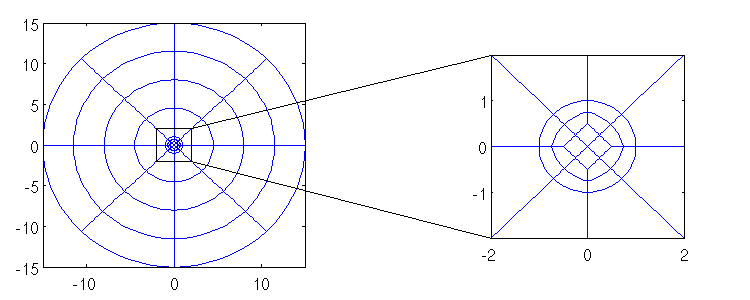Mesh output

Matlab plots of the total field : 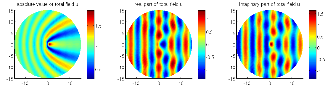Matlab output

References

[1] A. Bayliss, M. Gunzburger, and E. Turkel, "Boundary conditions for the numerical solution of elliptic equations in exterior domains", SIAM J. Appl. Math., vol. 42, no. 2, pp. 430-451, 1982.

Complete Source Code

Author: Dirk Klindworth, 2011

#include <iostream>
 
#include "basics.hh"
#include "formula.hh"
#include "function.hh"
#include "geometry.hh"
#include "graphics.hh"
#include "hp1D.hh"
#include "hp2D.hh"
#include "operator.hh"
#include "space.hh"
#include "toolbox.hh"
 
using concepts::Real;
using concepts::Cmplx;
 
int main(int argc, char** argv) {
  try {
 
#ifdef HAS_MPI
    // Initialisation is necessary if parallel version of Mumps is compiled
    MPI_Init(&argc, &argv);
#endif
    
    // ** parameters **
    const Real  R      = 15.0;       // outer radius
    const Real  innerR =  1.0;       // inner radius (i.e. radius of scatterer)
    const Real  omega  =  1.0;       // frequency
    const Real  eps0   =  1.0;       // permittivity outside the scatterer
    const Real  mu0    =  1.0;       // permeability outside the scatterer
    const Cmplx epsSc    (4.0, 0.0); // permittivity inside the scatterer
    const Real  muSc   =  1.0;       // permeability inside the scatterer
    
    // ** attributes of the computational domain **
    const uint attrBoundary = 11;    // boundary
    const uint attrSc       = 21;    // scatterer
    const uint attr0        = 22;    // computational domain without scatterer
    
    // ** set mode **
    enum TETM {TE, TM};
    TETM mode = TM;
    
    // ** declare piecewise constant formulas for alpha and beta **
    concepts::PiecewiseConstFormula<Cmplx> alpha;
    concepts::PiecewiseConstFormula<Cmplx> beta;
    concepts::ConstFormula<Cmplx>          alpha0;
    
    // ** Piecewise constant alpha and beta (TE-case) **
    if (mode == TE) {
      alpha[concepts::Attribute(attrSc)] = Cmplx(pow(epsSc,-1.0));
      alpha[concepts::Attribute(attr0)]  = Cmplx(pow(eps0,-1.0),0.0);
      beta[concepts::Attribute(attrSc)] = Cmplx(omega*omega*muSc,0.0);
      beta[concepts::Attribute(attr0)]  = Cmplx(omega*omega*mu0,0.0);
      alpha0 = Cmplx(pow(eps0,-1.0),0.0);
    }
    
    // ** Piecewise constant alpha and beta (TM-case) **
    if (mode == TM) {
      alpha[concepts::Attribute(attrSc)] = Cmplx(1.0, 0.0);
      alpha[concepts::Attribute(attr0)]  = Cmplx(1.0, 0.0);
      beta[concepts::Attribute(attrSc)] = Cmplx(omega*omega*epsSc*muSc);
      beta[concepts::Attribute(attr0)]  = Cmplx(omega*omega*eps0*mu0,0.0);
      alpha0 = Cmplx(1.0, 0.0);
    }
    
    // ** wave vector in the exterior **
    const Real k0 = omega*sqrt(mu0*eps0);
    
    // ** BGT-0 coefficient **
    const Cmplx BGTcoeff(0.0,k0);
    
    // ** incoming wave, its normal gradient and its product with the BGT-0 coefficient **
    std::stringstream uIncReal, uIncImag, uIncGradReal, uIncGradImag, uIncBGTReal, uIncBGTImag;
    uIncReal     << "(cos((" << k0 << ")*x))";
    uIncImag     << "(sin((" << k0 << ")*x))";
    uIncGradReal << "(-(x/(sqrt(x*x+y*y)))*" << k0 << "*sin((" << k0 << ")*x))";
    uIncGradImag << "( (x/(sqrt(x*x+y*y)))*" << k0 << "*cos((" << k0 << ")*x))";
    uIncBGTReal  << "(" << real(BGTcoeff) << "*" << uIncReal.str() << "-" << imag(BGTcoeff) << "*" << uIncImag.str() << ")";
    uIncBGTImag  << "(" << real(BGTcoeff) << "*" << uIncImag.str() << "+" << imag(BGTcoeff) << "*" << uIncReal.str() << ")";
    concepts::ParsedFormula<Cmplx>     uInc(    uIncReal.str(),     uIncImag.str());
    concepts::ParsedFormula<Cmplx> uIncGrad(uIncGradReal.str(), uIncGradImag.str());
    concepts::ParsedFormula<Cmplx>  uIncBGT( uIncBGTReal.str(),  uIncBGTImag.str());
 
    // ** create mesh **
    Real ringData[3]     = {innerR,(innerR+R)/2.0,R};
    uint quadAttrData[3] = {attrSc,attr0,attr0};
    uint edgeAttrData[3] = {0,0,attrBoundary};
    concepts::Array<Real> ring(ringData,3);
    concepts::Array<uint> ringQuadAttr(quadAttrData,3);
    concepts::Array<uint> ringEdgeAttr(edgeAttrData,3);
    concepts::Circle msh(ring,ringQuadAttr,ringEdgeAttr);
    std::cout << std::endl << "Mesh: " << msh << std::endl;
    graphics::drawMeshEPS(msh,"BGT_0_mesh.eps",100,1.0,20);
    
    // ** space **
    hp2D::Space spc(msh, 1, 10);
    spc.rebuild();
    std::cout << std::endl << "Space: " << spc << std::endl;
    graphics::drawMeshEPS(spc,"BGT_0_space.eps",100,1.0,20); 
    
    // ** build trace space of boundary **
    hp2D::TraceSpace tspc(spc,concepts::makeSet<uint>({attrBoundary}),hp2D::TraceSpace::FIRST);
    std::cout << std::endl << "Trace Space: " << tspc << std::endl;
    
    // ** right hand side **
    hp1D::Riesz<Cmplx> lform(alpha0*uIncGrad - alpha0*uIncBGT);
    concepts::Vector<Cmplx> rhs(tspc, lform);
    
    // ** system matrix **
    concepts::SparseMatrix<Cmplx> S(spc.dim(), spc.dim());
    hp2D::Laplace<Cmplx> la(alpha);
    concepts::SparseMatrix<Cmplx> A(spc, la);
    A.addInto(S, 1.0);
    hp2D::Identity<Cmplx> id2D(beta);
    concepts::SparseMatrix<Cmplx> M2D(spc, id2D);
    M2D.addInto(S, -1.0);
    hp1D::Identity<Cmplx> id1D(alpha0);
    concepts::SparseMatrix<Cmplx> M1D(tspc, id1D);
    M1D.addInto(S, -BGTcoeff);
    std::cout << std::endl << "System Matrix: " << S << std::endl;
    
    // ** solve **
#ifdef HAS_MUMPS
    concepts::Mumps<Cmplx> solver(S);
#else
    concepts::SuperLU<Cmplx> solver(S);
#endif
 
    std::cout << std::endl << "Solver: " << solver << std::endl;
    concepts::Vector<Cmplx> sol(spc);
    solver(rhs, sol);
    std::cout << " ... solved " << std::endl;    
    
    // ** plot solution **  
    hp2D::IntegrableQuad::factory().get()->setTensor(concepts::TRAPEZE, true, 10);
    spc.recomputeShapefunctions();
    graphics::MatlabBinaryGraphics(spc, "BGT_0", sol);
    
  }
  catch (concepts::ExceptionBase& e) {
    std::cout << e << std::endl;
    return 1;
  }
 
#ifdef HAS_MPI
  MPI_Finalize();
#endif
 
  return 0;
}

A function class to calculate element matrices for the mass matrix.

Definition: bilinearForm.hh:64

hp2D::TraceSpace

Builds the trace space of an FE space.

Definition: traces.hh:52

concepts::PiecewiseConstFormula

Piecewise constant function defined by the attribute of a cell.

Definition: formula.hh:84

hp2D::IntegrableQuad::factory

static std::unique_ptr< concepts::QuadRuleFactoryTensor2d > & factory()

Access to the quadrature rule, which is valid for all elements of this type (hp2D::IntegrableQuad).

Definition: quad.hh:145

concepts::TRAPEZE

@ TRAPEZE

Definition: defines.hh:13

concepts::SuperLU

Direct sparse solver for unsymmetric matrices.

Definition: superLU.hh:70

concepts::ConstFormula

Class for a constant formula.

Definition: constFormula.hh:26

concepts::ExceptionBase

Base class for exceptions.

Definition: exceptions.hh:86

graphics::drawMeshEPS

MeshEPS< Real > drawMeshEPS(concepts::Mesh &msh, std::string filename, const Real scale=100, const Real greyscale=1.0, const unsigned int nPoints=2)

Trampoline function to create a MeshEPS.

concepts::ParsedFormula< Cmplx >

Definition: parsedFormula.hh:113

concepts::SparseMatrix::addInto

void addInto(Matrix< H > &dest, const I fact, const uint rowoffset=0, const uint coloffset=0) const

This matrix is added as block to the given matrix dest.

Definition: sparseMatrix.hh:538

A function class to calculate element matrices for the mass matrix.

Definition: bf_identity.hh:58

Linear form on edges in nD.

Definition: linearForm.hh:67

hp2D::Space::rebuild

Space rebuild()

Rebuilds the space.

concepts::Array< Real >

graphics::MatlabBinaryGraphics

Class that allows to store graphical infomations in .mat files to use them in Matlab.

Definition: matlabBinaryGraphics.hh:28

concepts::Cmplx

std::complex< Real > Cmplx

Type for a complex number. It also depends on the setting of Real.

Definition: typedefs.hh:39

concepts::Vector< Cmplx >

hp2D::Space::dim

virtual uint dim() const

Definition: space.hh:393

hp2D::Space::recomputeShapefunctions

void recomputeShapefunctions()

Recompute shape functions, e.g.

double beta(const double a, const double b)

A function class to calculate element matrices for the Laplacian.

Definition: bf_laplace.hh:91

A 2D hp FEM space with continuous, piecewise polynomial basis functions.

Definition: space.hh:88

concepts::Mumps

MUMPS : MUltifrontal Massively Parallel sparse direct Solver.

Definition: mumps.hh:72

hp2D::TraceSpace::FIRST

@ FIRST

Definition: traces.hh:57

concepts::Circle

Mesh for a circle.

Definition: circle.hh:47

concepts::Attribute

Attributes for elements of the topology.

Definition: connector.hh:22

double Real

Type normally used for a floating point number.

Definition: typedefs.hh:36

concepts::SparseMatrix

Sparse matrix.

Definition: compositions.hh:25

Page URL: http://wiki.math.ethz.ch/bin/view/Concepts/WebHome
21 August 2020
© 2020 Eidgenössische Technische Hochschule Zürich