Introduction
This tutorial is very similar to the two dimensional hp-FEM tutorial in hpFEM2d.cc; you should have read it to understand this tutorial.
Maxwell's Equations
The equations solved are the time-harmonic Maxwell's equations:
![\[ - \varepsilon i \omega \vec E + \text{curl} \vec H = \sigma \vec E + \vec J \]](form_153.png)
![\[ \mu i \omega \vec H + \text{curl} \vec E = 0 \]](form_154.png)
with the divergence conditions (assuming no charge density)
![\[ \text{div} \mu \vec H = 0 \qquad \text{and} \qquad \text{div} \varepsilon \vec E = 0. \]](form_155.png)
Extracting  from the second equation and inserting in into the first formally yields
![\[ \text{curl}( \mu^{-1} \text{curl} \vec E) - \omega^2 (\varepsilon + \frac{\sigma}{i\omega}) \vec E = -i \omega \vec J, \]](form_157.png)
the so-called electric source problem. The appropriate space is
![\[ H(\text{curl}; D) := \{\vec u \in L^2(D)^3 : \text{curl} \vec u \in L^2(D)^3 \}. \]](form_158.png)
However, the curl-curl form above is not defined for electric fields in  . This is resolved in the variational formulation of the electric source problem:
Find  such that
![\[ \int_D (\mu^{-1} \text{curl} \vec E \cdot \text{curl} \vec v - \omega^2 \tilde\varepsilon \vec E \cdot \vec v) \, d\vec x = \int_D \vec f \cdot \vec v \, d\vec x \quad \forall \vec v \in H_0(\text{curl}; D), \]](form_161.png)
where  is
is  with the prefect conductor boundary conditions
  ,
,  and
and  . The associated bilinear operator of this variational formulation is not elliptic and the divergence condition is an independent constraint. Normally, Maxwell's equations are discretised using Nedelec's elements. However, there are good reasons why one would like to use standard H1-conforming FEM. This is possible using weighted regularization.
Weighted Regularization
The divergence can be forced to zero by adding
![\[ \int_D \text{div} \vec E \text{div} \vec v \, d\vec x \]](form_166.png)
to the bilinear form. However, this works only in non-convex domains. With the weighted regularization and the new bilinear form
![\[ \int_D (\mu^{-1} \text{curl} \vec E \cdot \text{curl} \vec v - \omega^2 \tilde\varepsilon \vec E \cdot \vec v) \, d\vec x + \langle\text{div}\vec E, \text{div}\vec v\rangle_Y \]](form_167.png)
where  and
and
![\[ X_n[Y] := \{\vec u \in H_0(\text{curl}; D): \text{div}\vec u \in Y\} \]](form_169.png)
is dense in  (the space we are discretising with H1-conforming FEM). A simple choice for the weight
  in three dimensions is
![\[ w(\vec x) = \text{dist}\left( \vec x, \bigcup_{c \in C} c \cup \bigcup_{e \in E} \bar e \right), \]](form_172.png)
where  is the set of reentrant corners and
  the set of reentrant edges. Then,
![\[ \langle\text{div} \vec u, \text{div} \vec v\rangle_Y = \int_D w^2 \text{div} \vec u \text{div} \vec v \, d\vec x. \]](form_175.png)
- See also
- Martin Costabel and Monique Dauge. Weighted regularization of Maxwell equations in polyhedral domains. A rehabilitation of nodal finite elements. Numer. Math., 93(2):239-277, 2002.
Maxwell Eigenproblem
The Maxwell Eigenproblem is solved using the weighted regularization:
Find frequencies  and functions
 ![$0 \neq \vec E \in X_n[Y]$](form_177.png) such that
such that
![\[ \int_D \mu^{-1} \text{curl}\vec E \cdot \text{curl} \vec v\, d\vec x + s\langle\text{div} \vec E, \text{div} \vec v\rangle_Y = \omega^2 \int_D \varepsilon \vec E \cdot \vec v \, d\vec x \quad \forall \vec v \in X_n[Y]. \]](form_178.png)
The necessary FE spaces are built using vectorial::Space and hp3D::Space. The bilinear forms are built with hp3D::RotRot, hp3D::DivDiv and vectorial::BilinearForm and hp3D::Identity.
Contents
- Commented Program
-
FEM Routine
-
Main Program
- Results
- Complete Source Code
Commented Program
As said above, this tutorial is very similar in large parts to hpFEM2d.cc and the documentation below is terser (ie. only new stuff is commented).
#include <cmath>
#include <cstdlib>
#include <iostream>
#include <sstream>
#include <memory>
#include <fstream>
#include <unistd.h>
#include "function.hh"
#include "graphics.hh"
#include "integration.hh"
#include "operator.hh"
#include "space.hh"
The new includes files are hp3D.hh for the three dimensional hp-FEM, vectorial.hh for the classes to build vector valued FE spaces etc. from the scalar components and eigensolver.hh for the Eigensolvers needed below.
FEM Routine
Most abbreviations are the same (including the same meaning) as already known.
const uint l = input.
getInt(
"level");
const uint p = input.
getInt(
"polynomial");
const std::string meshNameBase = input.
getString(
"meshNameBase");
New parameters to configure the Eigensolvers are kmax (how many Eigenvalues should be computed at the same time), solverType (which type of Eigensolver, there are a few available) and shift (parameter  for the shift-invert method).
const uint kmax = input.
getInt(
"kmax");
The following parameters are used for the weighted regularization: rho is to distinguish physical from spurious Eigenvalues by the following criterion (using the Eigenfunction  ):
):
![\[ \frac{\|\text{curl} \vec E\|^2_0}{s \|\text{div} \vec E\|_Y^2} \begin{cases} \geq \rho & \text{physical Eigenvalue} \\ \leq \rho^{-1} & \text{spurious Eigenvalue} \\ \text{otherwise} & \text{undecided}. \end{cases} \]](form_181.png)
A good value for rho is 1.5 (the default).
weight is used to choose one of various weights (including different weigth exponents (instead of 2 as in the introduction).
const uint weight = input.
getInt(
"weight");
Then, the array for the values of the scaling parameter s are set up.
const uint sNumber = input.
getInt(
"sNumber");
for (uint i = 0; i < sNumber; ++i) s[i] = input.
getArrayDouble(
"s", i);
Mesh
std::stringstream fileCoord;
fileCoord << meshNameBase << "Coord.dat" << std::ends;
output.
addString(
"coordFile", fileCoord.str().c_str());
std::stringstream fileElements;
fileElements << meshNameBase << "Elements.dat" << std::ends;
output.
addString(
"elementsFile", fileElements.str().c_str());
std::stringstream fileBoundary;
fileBoundary << meshNameBase << "Boundary.dat" << std::ends;
output.
addString(
"boundaryFile", fileBoundary.str().c_str());
fileBoundary.str());
std::cout << "Mesh: " << msh << std::endl;
Space
The perfect conductor boundary conditions  can be set up by carefully choosing the Dirichlet boundary conditions of the three scalar components of the vector valued FE space.
Finally, the FE spaces can be set up. First, a vector valued FE space with three components is created. This is essentially a container (as most of the classes of vectorial) which takes care of different scalar components which can be added to it.
Then, one after the other scalar FE space is created and added to the vector valued FE space spc. Note that the scalar FE spaces have to be rebuilt before adding them to spc. This call to hp3D::Space::rebuild creates the elements.
hp3D::Space sspcX(msh, 0, p, &bcX); sspcX.rebuild(); spc.put(sspcX);
hp3D::Space sspcY(msh, 0, p, &bcY); sspcY.rebuild(); spc.put(sspcY);
hp3D::Space sspcZ(msh, 0, p, &bcZ); sspcZ.rebuild(); spc.put(sspcZ);
for (uint i = 0; i < l; ++i) {
std::cout << "i = " << i << std::endl;
The scalar spaces also have to be rebuilt separately after a refinement before rebuilding the vector valued space.
sspcX.rebuild();
std::cout << " scalar space: " << std::flush;
std::cout << sspcX << std::endl;
Computations
The stiffness matrix has two parts: rot-rot and div-div. These two parts are built separately. Before calling the Eigensolver, a linear combination depending on s of the two is created. The classes hp3D::RotRot and hp3D::DivDiv both come with a setup routine to take care of some technicalities. The use of this routine is not mandatory but recommended.
The rot-rot part of the stiffness matrix is simple to compute.
rotrot.compress();
std::cout << " rot rot matrix: " << rotrot << std::endl;
The div-div part of the stiffness matrix is somewhat more involved: the singularities of the solutions have to be taken into account by the weight. The singular edes and vertices are marked, this information is later used by the div-div bilinear form.
Various weights can be selected on the command line or via the input file. This is reflected in weight.
switch (weight) {
case 0:
break;
case 1:
break;
case 11:
break;
case 21:
break;
}
std::cout << " div div bilinear form: "
<< *(vdivdiv_bf.get(0)) << std::endl;
std::stringstream weightName;
weightName << *(vdivdiv_bf.get(0));
output.
addString(
"weight", weightName.str().c_str());
After having selected the right bilinear form (the right weight for the div-div form), the div-div stiffness matrix can be computed
divdiv.compress();
std::cout << " div div matrix: " << divdiv << std::endl;
The mass matrix consists of three scalar mass matrices in the diagonal blocks of the mass matrix. They are put together in the canonical way to build a vector valued bilnear form.
Each call to vectorial::BilinearForm::put adds a scalar bilinear form into a block of the vector valued bilinear form. In this case, only the diagonal blocks have to be filled.
mass_bf.put(smass_bf, 0, 0);
mass_bf.put(smass_bf, 1, 1);
mass_bf.put(smass_bf, 2, 2);
std::cout << " mass matrix: " << mass << std::endl;
mass.compress();
std::cout << " mass matrix: " << mass << std::endl;
The next step is to set up the solver. There is loop over the different values of the scaling parameter s around the solution process.
for (uint sIndex = 0; sIndex < sNumber; ++sIndex) {
std::cout << " s = " << s[sIndex] << std::endl;
The Eigensolver shall be constructed by a fabric, ie. a class derived from eigensolver::SolverFabric. solverType contains which solver to use and it is evaluated in the following switch case clause.
After having chosen the solver by creating the appropriate fabric, the solver can be instantiated.
A call to eigensolver::Solver::getEV returns the Eigenvalues. They are printed to screen in a list.
Postprocessing
Then, a list of the Eigenvalues together with the categorization (the formula is given above) is printed to screen. In addition, the Eigenvalue together with the rotrot energy and the divdiv energy are stored in the output data for later postprocessing (or plotting).
Compute the rotrot energy: 
Compute the divdiv energy: 
Evaluate the criterion and print the results.
Finally, the data is stored in output.
Refinement of the Space
Each component of the vector valued space has to be refined individually towards the singularly marked vertices and edges.
Main Program
The main program works very similar to the previous tutorials.
Command Line Arguments
The arrays to store the Eigenvalues and the divdiv and rotrot energies have to be prepared.
Results
To restrict the amount of output, we are calling the program with the following input file:@code int level 1 int kmax 3 int sNumber 1 array double s { 0 2.0 } Then, the output looks like:
[./hpFEM3d-EV]
--
Parameters:
input file = t.concepts
string author "(empty)"
string comment "(empty)"
string gnuplot "./hpFEM3d-EV.gnuplot"
string meshNameBase "../../../applications/thickLshape"
string parameterout "./hpFEM3d-EV.out"
string title "Maxwell Eigenvalues in 3D using weighted regularization"
int edgRef 77
int faceRef 0
int kmax 3
int level 1
int polynomial 2
int sNumber 1
int solver 2
int vtxRef 66
int weight 11
double rho 1.5
double shift 9
array double s {
0 2
1 2
2 3
3 4
4 20
5 9
6 12
7 15
8 17
9 30
}
--
Mesh: Import3dMesh(ncell = 3)
i = 0
scalar space: Space(dim = 7, nelm = 3)
Space(dim = 7, nelm = 3)
Space(dim = 12, nelm = 3)
vector valued space (3 comp.): Space(idx = 3, vdim = 3, dim = 26, nelm = 3)
rot rot matrix: SparseMatrix(26x26, HashedSparseMatrix: 316 (46.7456%) entries bound.)
div div bilinear form: DivDiv(weight = ProductOfAll)
div div matrix: SparseMatrix(26x26, HashedSparseMatrix: 334 (49.4083%) entries bound.)
mass matrix: SparseMatrix(26x26, HashedSparseMatrix: 426 (63.0178%) entries bound.)
mass matrix: SparseMatrix(26x26, HashedSparseMatrix: 158 (23.3728%) entries bound.)
s = 2
solver = ArPack(shift-invert mode(3), not yet computed largest (algebraic) eigenvalues, sigma = 9, n = 26, tol = 0, conv. eigenpairs = 0(max = 3), Arnoldi iter = 0(max = 1000), 0 OP*x ops., 0 B*x ops., 0 steps of re-orth.)
Eigenvalues: Array<F>(3, [9.90411138346484, 14.167902552732, 14.5499375050742])
solver = ArPack(shift-invert mode(3), computed largest (algebraic) eigenvalues, sigma = 9, n = 26, tol = 1.11022302462516e-16, conv. eigenpairs = 3(max = 3), Arnoldi iter = 13(max = 1000), 34 OP*x ops., 112 B*x ops., 33 steps of re-orth.)
EV 0 = 9.90411138346484 has rotEnergy = 9.9041, divEnergy*s = 7.1322e-32, L2
norm = 1
EV 1 = 14.167902552732 has rotEnergy = 13.806, divEnergy*s = 0.36222, L2
norm = 1
EV 2 = 14.5499375050742 has rotEnergy = 13.526, divEnergy*s = 1.0238, L2
norm = 1
--
Writing gathered data to disk: ./hpFEM3d-EV.out
The mesh normally used is a thick L shaped domain in three hexahedra. The mesh looks like this: 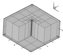 With 18726 dofs, the Eigenvalues plotted versus s:
 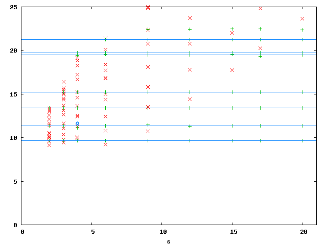 The physical Eigenvalues (green) are lined up on horizontal lines whereas the spurious Eigenvalues are on straight lines through the origin. The exact values (horizontal blue lines) are taken from Monique Dauge's Benchmax page. Below are the convergence histories for the first three Eigenvalues for selected values of s:
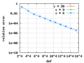
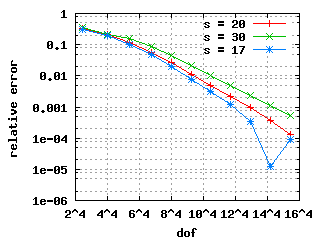
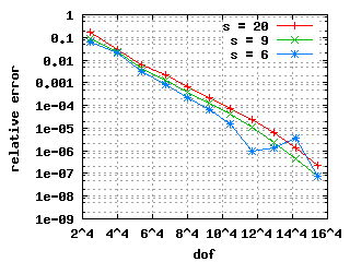 These convergence histories show exponential convergence: straight lines in a
 ![$ \log-\sqrt[4]{.} $](form_184.png) plot.
plot.
Complete Source Code
- Author
- Philipp Frauenfelder, 2004
#include <cmath>
#include <cstdlib>
#include <iostream>
#include <sstream>
#include <memory>
#include <fstream>
#include <unistd.h>
#include "function.hh"
#include "graphics.hh"
#include "integration.hh"
#include "operator.hh"
#include "space.hh"
#include "vectorial.hh"
const uint l = input.
getInt(
"level");
const uint p = input.
getInt(
"polynomial");
const std::string meshNameBase = input.
getString(
"meshNameBase");
const uint kmax = input.
getInt(
"kmax");
const uint weight = input.
getInt(
"weight");
const uint sNumber = input.
getInt(
"sNumber");
for (uint i = 0; i < sNumber; ++i) s[i] = input.
getArrayDouble(
"s", i);
std::stringstream fileCoord;
fileCoord << meshNameBase << "Coord.dat" << std::ends;
output.
addString(
"coordFile", fileCoord.str().c_str());
std::stringstream fileElements;
fileElements << meshNameBase << "Elements.dat" << std::ends;
output.
addString(
"elementsFile", fileElements.str().c_str());
std::stringstream fileBoundary;
fileBoundary << meshNameBase << "Boundary.dat" << std::ends;
output.
addString(
"boundaryFile", fileBoundary.str().c_str());
fileBoundary.str());
std::cout << "Mesh: " << msh << std::endl;
const uint vdim = 3;
for (uint i = 0; i < l; ++i) {
std::cout << "i = " << i << std::endl;
std::cout << " scalar space: " << std::flush;
std::cout << sspcX << std::endl;
std::cout << " " << sspcY << std::endl;
std::cout << " " << sspcZ << std::endl;
spc.rebuild();
std::cout << " vector valued space (" << vdim << " comp.): "
<< std::flush;
std::cout << spc << std::endl;
if (spc.dim() > 20) {
std::cout << " rot rot matrix: " << rotrot << std::endl;
switch (weight) {
case 0:
break;
case 1:
break;
case 11:
break;
case 21:
break;
}
std::cout << " div div bilinear form: "
<< *(vdivdiv_bf.get(0)) << std::endl;
std::stringstream weightName;
weightName << *(vdivdiv_bf.get(0));
output.
addString(
"weight", weightName.str().c_str());
std::cout << " div div matrix: " << divdiv << std::endl;
mass_bf.
put(smass_bf, 0, 0);
mass_bf.
put(smass_bf, 1, 1);
mass_bf.
put(smass_bf, 2, 2);
std::cout << " mass matrix: " << mass << std::endl;
std::cout << " mass matrix: " << mass << std::endl;
for (uint sIndex = 0; sIndex < sNumber; ++sIndex) {
std::cout << " s = " << s[sIndex] << std::endl;
if (sIndex == 0)
const uint nEV = sol_eigenvalue.
size();
std::cout.precision(15);
std::cout << " Eigenvalues: " << sol_eigenvalue << std::endl;
for (uint evIndex = 0; evIndex < nEV; ++evIndex) {
rotrot(*(sol_eigenfunction[evIndex]), tmp);
Real rotEnergy = real(*(sol_eigenfunction[evIndex]) * tmp);
divdiv(*(sol_eigenfunction[evIndex]), tmp);
Real divEnergy = real(*(sol_eigenfunction[evIndex]) * tmp) * s[sIndex];
std::string quality;
if ( std::fabs(rotEnergy)/std::fabs(divEnergy) >= rho) {
quality = "**";
} else {
if ( std::fabs(rotEnergy)/std::fabs(divEnergy) <= 1./rho)
quality = " ";
else quality = " *";
}
std::cout << quality << " EV " << evIndex << " = ";
std::cout.precision(15);
std::cout << sol_eigenvalue[evIndex];
std::cout.precision(5);
mass(*(sol_eigenfunction[evIndex]), tmp);
Real L2norm = real(*(sol_eigenfunction[evIndex]) * tmp);
std::cout << " has rotEnergy = " << rotEnergy
<< ", divEnergy*s = " << divEnergy
<< ", L2 norm = " << L2norm
<< std::endl;
std::stringstream name1, name2, name3;
name1 << "ev_s_" << s[sIndex] << "_k_" << evIndex << std::ends;
sol_eigenvalue[evIndex].real());
name2 << "dE_s_" << s[sIndex] << "_k_" << evIndex << std::ends;
name3 << "rE_s_" << s[sIndex] << "_k_" << evIndex << std::ends;
}
}
}
if (i < l-1) {
int pMax[3] = { 1, 1, 1 };
for (uint j = 0; j < 3; ++j) {
(*spaces[j], input.
getInt(
"vtxRef"), input.
getInt(
"edgRef"),
input.
getInt(
"faceRef"), pMax);
post(refineSpace);
}
std::cout << "--" << std::endl;
}
}
}
int main(int argc, char** argv) {
try {
input.
addInt(
"polynomial", 2);
input.
addString(
"meshNameBase", SOURCEDIR
"/applications/thickLshape");
s[0] = 6;
s[1] = 2;
s[2] = 3;
s[3] = 4;
s[4] = 20;
s[5] = 9;
s[6] = 12;
s[7] = 15;
s[8] = 17;
s[9] = 30;
for (uint i = 0; i < (uint)input.
getInt(
"sNumber"); ++i)
"Maxwell Eigenvalues in 3D using weighted regularization");
std::stringstream outfile;
outfile << argv[0] << ".out" << std::ends;
input.
addString(
"parameterout", outfile.str().c_str());
std::stringstream gnuplotfile;
gnuplotfile << argv[0] << ".gnuplot" << std::ends;
input.
addString(
"gnuplot", gnuplotfile.str().c_str());
output.
addString(
"version",
"$Id: hpFEM3d-EV.cc,v 1.5 2005/08/26 15:35:48 kersten Exp $");
std::string inputfile;
int opt;
while ((opt = getopt(argc, argv, "-f:e:l:p:k:r:n:s:w:")) != EOF)
switch(opt) {
case 'l': input.
addInt(
"level", atoi(optarg));
break;
case 'p': input.
addInt(
"polynomial", atoi(optarg));
break;
case 'f': inputfile = std::string(optarg);
inputParser.
parse(inputfile);
break;
case 'e': input.
addInt(
"solver", std::atoi(optarg));
break;
case 'k': input.
addInt(
"kmax", std::atoi(optarg));
break;
case 'r': input.
addDouble(
"rho", std::atof(optarg));
break;
case 'n': input.
addString(
"meshNameBase", optarg);
break;
case 's': input.
addDouble(
"shift", std::atof(optarg));
break;
case 'w': input.
addInt(
"weight", std::atoi(optarg));
break;
default:
std::cout << "Option '" << opt << "' unkown." << std::endl
<< "Usage: " << argv[0]
<< " [-f FILE] [-l LEVEL] [-e SOLVER] [-k KMAX] [-p POLY] "
<< "[-r RHO] [-n MESH_NAME] [-s SHIFT] [-w WEIGHT]"
<< std::endl
<< "where" << std::endl
<< " FILE: name of the input file" << std::endl
<< " LEVEL: level of refinement" << std::endl
<< " SOLVER: JDBSYM(0), ARPACK(1)" << std::endl
<< " POLY: starting polynomial degree" << std::endl
<< " KMAX: number of eigenvalues which should be computed"
<< std::endl
<< " MESH_NAME: name of the mesh (thickLshape)" << std::endl
<< " SHIFT: shift for Eigenvalue solver" << std::endl
<< " WEIGHT:" << std::endl
<< " 0: TrivialWeight" << std::endl
<< " 1: ShortestDist" << std::endl
<< " 11: ProductOfAll" << std::endl
<< " 21: DaugeWeight" << std::endl
<< "Options given after the input file override the values "
<< "read from the"
<< std::endl << "input file." << std::endl;
exit(1);
break;
}
for (uint i = 0; i < (uint)input.
getInt(
"sNumber"); ++i) {
for (uint j = 0; j < (uint)input.
getInt(
"kmax"); ++j) {
std::stringstream name1, name2, name3;
<< std::ends;
output);
<< std::ends;
output);
<< std::ends;
output);
}
}
std::cout << '[' << argv[0] << "]" << std::endl;
std::cout << "--" << std::endl;
std::cout << "Parameters:" << std::endl
<< " input file = " << inputfile << std::endl
<< input;
std::cout << "--" << std::endl;
fem(input, output);
std::ofstream* ofs = new std::ofstream
(input.getString("gnuplot").c_str());
*ofs << std::setprecision(20);
delete ofs;
std::cout << " --" << std::endl
<< " Writing gathered data to disk: "
<< input.getString("parameterout") << std::endl;
ofs = new std::ofstream(input.getString("parameterout").c_str());
*ofs << "/* program:\t" << argv[0] << std::endl
<< " * command:\t";
for (int j = 0; j < argc; ++j)
*ofs << argv[j] << " ";
*ofs << std::endl
<< " * input file:\t" << inputfile << std::endl;
*ofs << " */" << std::endl << std::setprecision(20) << inputParser;
delete ofs;
}
std::cout << e << std::endl;
return 1;
}
return 0;
}
![]()
![]()
![]()
![]() from the second equation and inserting in into the first formally yields
from the second equation and inserting in into the first formally yields ![]()
![]()
![]() . This is resolved in the variational formulation of the electric source problem:
. This is resolved in the variational formulation of the electric source problem: ![]() such that
such that ![]()
![]() is
is ![]() with the prefect conductor boundary conditions
with the prefect conductor boundary conditions ![]() ,
, ![]() and
and ![]() . The associated bilinear operator of this variational formulation is not elliptic and the divergence condition is an independent constraint. Normally, Maxwell's equations are discretised using Nedelec's elements. However, there are good reasons why one would like to use standard H1-conforming FEM. This is possible using weighted regularization.
. The associated bilinear operator of this variational formulation is not elliptic and the divergence condition is an independent constraint. Normally, Maxwell's equations are discretised using Nedelec's elements. However, there are good reasons why one would like to use standard H1-conforming FEM. This is possible using weighted regularization.![]()
![]()
![]() and
and ![]()
![]() (the space we are discretising with H1-conforming FEM). A simple choice for the weight
(the space we are discretising with H1-conforming FEM). A simple choice for the weight ![]() in three dimensions is
in three dimensions is ![]()
![]() is the set of reentrant corners and
is the set of reentrant corners and ![]() the set of reentrant edges. Then,
the set of reentrant edges. Then, ![]()
![]() and functions
and functions ![]() such that
such that ![]()
![]() for the shift-invert method).
for the shift-invert method). ![]() ):
): ![\[ \frac{\|\text{curl} \vec E\|^2_0}{s \|\text{div} \vec E\|_Y^2} \begin{cases} \geq \rho & \text{physical Eigenvalue} \\ \leq \rho^{-1} & \text{spurious Eigenvalue} \\ \text{otherwise} & \text{undecided}. \end{cases} \]](form_181.png)
![]() can be set up by carefully choosing the Dirichlet boundary conditions of the three scalar components of the vector valued FE space.
can be set up by carefully choosing the Dirichlet boundary conditions of the three scalar components of the vector valued FE space. ![]()
![]()
 With 18726 dofs, the Eigenvalues plotted versus s:
  The physical Eigenvalues (green) are lined up on horizontal lines whereas the spurious Eigenvalues are on straight lines through the origin. The exact values (horizontal blue lines) are taken from Monique Dauge's Benchmax page. Below are the convergence histories for the first three Eigenvalues for selected values of s:

 These convergence histories show exponential convergence: straight lines in a
 ![]() plot.
plot. 
