| Brand | Soft | Rocky | Extreme |
|---|---|---|---|
| 1 | 1014, 1062, 1040 | 884, 929, 893 | 824, 778, 792 |
| 2 | 1095, 1116, 1127 | 818, 794, 820 | 642, 633, 692 |
4 Factorial Treatment Structure
4.1 Introduction
In the completely randomized designs that we have seen so far, the \(g\) different treatments had no special “structure”. In practice, treatments are often combinations of the levels of two or more factors. Think for example of a plant experiment using combinations of light exposure and fertilizer, with yield as response. We call this a factorial treatment structure or a factorial design. If we observe all possible combinations of the levels of two or more factors, we call them crossed. An illustration of two crossed factors can be found in Table 4.1.
| Exposure / Fertilizer | Brand 1 | Brand 2 |
|---|---|---|
| low | x | x |
| medium | x | x |
| high | x | x |
With a factorial treatment structure, we typically have questions about both factors and their possible interplay:
- Does the effect of exposure (on the expected value of yield) depend on brand (or vice versa)? In other words, is the exposure effect brand-specific?
If the effects do not depend on the other factor, we could also ask:
What is the effect of changing exposure from, e.g., low to medium on the expected value of yield?
What is the effect of changing the brand on the expected value of yield?
Let us have a detailed look at another example: A lab experiment was performed to compare mountain bike tires of two different brands, 1 and 2. To this end, the tires were put on a simulation machine allowing for three different undergrounds (soft, rocky and extreme). Each combination of brand and underground was performed three times (using a new tire each time). The response was the driven kilometers until tread depth was reduced by a pre-defined amount. The experiments have been performed in random order. The data can be found in Table 4.2.
Clearly, brand and underground are crossed factors. We have three observations for every combination of the levels of brand and underground.
We first read the data (here, the data is already available as an R-object) and make sure that all categorical variables are correctly encoded as factors.
book.url <- "https://stat.ethz.ch/~meier/teaching/book-anova"
bike <- readRDS(url(file.path(book.url, "data/bike.rds")))
str(bike)
## 'data.frame': 18 obs. of 3 variables:
## $ brand : Factor w/ 2 levels "1","2": 1 1 1 1 1 1 ...
## $ underground: Factor w/ 3 levels "soft","rocky",..: 1 1 1 2 2 2 ...
## $ dist : num 1014 1062 1040 ...With R, we can easily count the observations with the function xtabs.
xtabs(~ brand + underground, data = bike)## underground
## brand soft rocky extreme
## 1 3 3 3
## 2 3 3 3The formula “~ brand + underground” in xtabs reads as “count the number of observations for every combination of the levels of the two factors brand and underground.”
Typical questions could be as follows:
- Does the effect of brand on the expected value of the distance depend on the underground, or vice versa?
If the effects do not depend on the other factor, we could also ask:
What is the effect of changing the underground from, e.g., soft to rocky on the expected value of the distance?
What is the effect of changing the brand from 1 to 2 on the expected value of the distance?
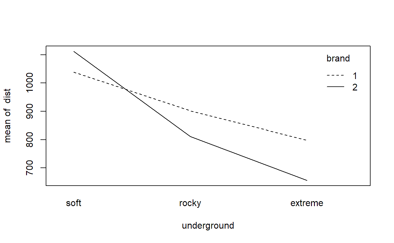
We can visualize such kind of data with a so-called interaction plot using the function interaction.plot. For every combination of the levels of brand (1 and 2) and underground (soft, rocky and extreme), we calculate the average value of the response (here, dist). We use underground on the \(x\)-axis (the first argument, also called x.factor). In addition, settings corresponding to the same level of brand are connected with lines (argument trace.factor). The role of underground and brand can of course also be interchanged. Hence, what factor we use as x.factor or as trace.factor is a question of personal preference. Most often it is natural to use an ordered factor as the x.factor, as we just did.
## elegant way, using the function "with"
with(bike, interaction.plot(x.factor = underground,
                            trace.factor = brand, response = dist))
## standard way: interaction.plot(x.factor = bike$underground,
##                                trace.factor = bike$brand,
## response = bike$dist)In Figure 4.1 we can observe that the average value of distance decreases when changing the underground from soft to rocky to extreme. This holds true for both brands. However, the drop of brand 2 when moving from soft to rocky is more pronounced compared to brand 1. One disadvantage of an interaction plot is the fact that it only plots averages and we do not see the underlying variation of the individual observations anymore. Hence, we cannot easily conclude that the effects which we observe in the plot are statistically significant or not.
A more sophisticated version could be plotted with the package ggplot2 (Wickham 2016) where we plot both the individual observations and the lines (for interested readers only).
library(ggplot2)
ggplot(bike, aes(x = underground, y = dist, color = brand)) +
  geom_point() + stat_summary(fun = mean, geom = "line",
                              aes(group = brand)) +
  theme_bw()
With this plot, we immediately see that the effects are rather large compared to the variation of the individual observations. If we have many observations, we could also use boxplots for every setting instead of the individual observations.
Let us now set up a parametric model which allows us to make a statement about the uncertainty of the estimated effects.
4.2 Two-Way ANOVA Model
We assume a general setup with a factor \(A\) with \(a\) levels, a factor \(B\) with \(b\) levels and \(n\) replicates for every combination of \(A\) and \(B\), a balanced design. Hence, we have a total of \(N = a \cdot b \cdot n\) observations. In the previous example, \(A\) was brand with \(a = 2\), \(B\) was underground with \(b =3\) and we had \(n = 3\) replicates for each treatment combination. This resulted in a total of \(N = 18\) observations.
We denote by \(y_{ijk}\) the \(k\)th observed value of the response of the treatment formed by the \(i\)th level of factor \(A\) and the \(j\)th level of factor \(B\). In the previous example, \(y_{213}\) would be the measured distance for the third tire (\(k = 3\)) of brand 2 (\(i = 2\)) and underground soft (\(j = 1\)). Hence, \(y_{213} = 1127\).
We now have to set up a model for \(a \cdot b\) different cell means, or a mean for each treatment combination. Conceptually, we could set up a one-way ANOVA model and try to answer the previous questions with appropriate contrasts. However, it is easier to incorporate the factorial treatment structure directly in the model.
The two-way ANOVA model with interaction is \[ Y_{ijk} = \mu + \alpha_i + \beta_j + (\alpha \beta)_{ij} + \epsilon_{ijk} \tag{4.1}\] where
- \(\alpha_i\) is the main effect of factor \(A\) at level \(i\), \(i = 1, \ldots, a\).
- \(\beta_j\) is the main effect of factor \(B\) at level \(j\), \(j = 1, \ldots, b\).
- \((\alpha \beta)_{ij}\) is the interaction effect between \(A\) and \(B\) for the level combination \(i,j\) (it is not the product \(\alpha_i \beta_j\)).
- \(\epsilon_{ijk}\) are i.i.d. \(N(0, \sigma^2)\) errors, \(k=1, \ldots, n\).
The expected values for the different cells in the bike tire example can be seen in Table 4.3.
| Brand | Soft | Rocky | Extreme |
|---|---|---|---|
| 1 | \(\mu + \alpha_1 + \beta_1 + (\alpha \beta)_{11}\) | \(\mu + \alpha_1 + \beta_2 + (\alpha \beta)_{12}\) | \(\mu + \alpha_1 + \beta_3 + (\alpha \beta)_{13}\) |
| 2 | \(\mu + \alpha_2 + \beta_1 + (\alpha \beta)_{21}\) | \(\mu + \alpha_2 + \beta_2 + (\alpha \beta)_{22}\) | \(\mu + \alpha_2 + \beta_3 + (\alpha \beta)_{23}\) |
As usual, we’ll have to use a side constraint for the parameters. We will use the sum-to-zero constraint, but we will handle the technical details later (note that the following interpretation is valid under this side constraint).
The effects can be interpreted as follows:
Think of main effects as “average effects” on the expected value of the response when changing the level of a factor. If we consider again Table 4.2 or Table 4.3, the main effects tell us something about average effects when moving from row to row (main effect of brand) and from column to column (main effect of underground).
The interaction effect contains the “leftovers” after having considered the main effects: Are there cell-specific properties that cannot be explained well by the main effects? In that sense, the interaction effect measures how far the cell means differ from a main effects only model. Or in other words, the interaction effect captures cell-specific behavior that was not captured with only row and column effects. If the model contains an interaction effect, the effect of, e.g., factor \(B\) (underground) depends on the level of factor \(A\) (brand). Otherwise, the whole effect could have been captured by the corresponding main effect!
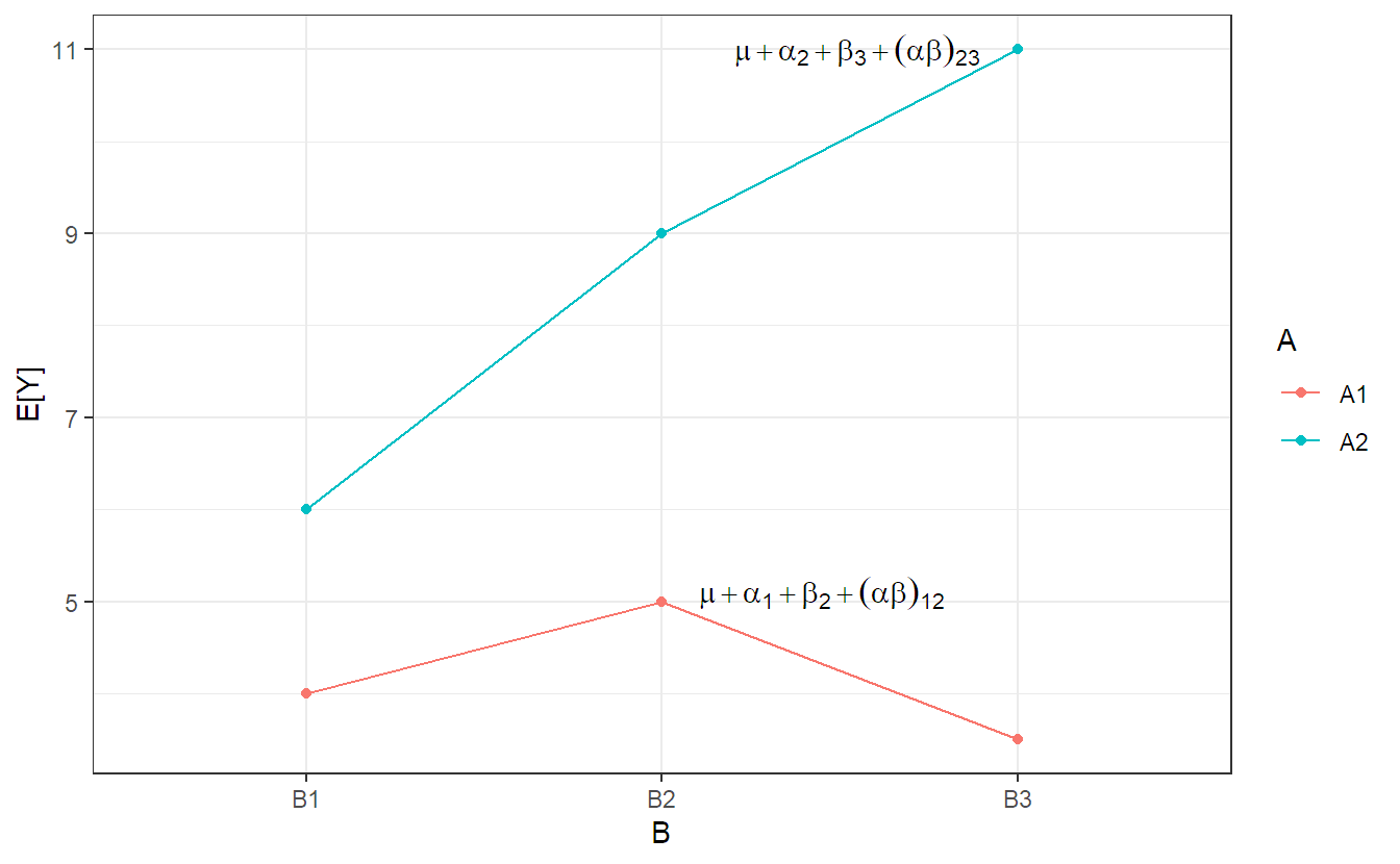
An illustration of the model, for a general setup, can be found in Figure 4.2. This plot is nothing more than a theoretical version of an interaction plot where we have the expected value instead of the sample average on the \(y\)-axis. We can observe that the model is flexible enough such that each treatment combination can get its very own mean value (“cell mean”).
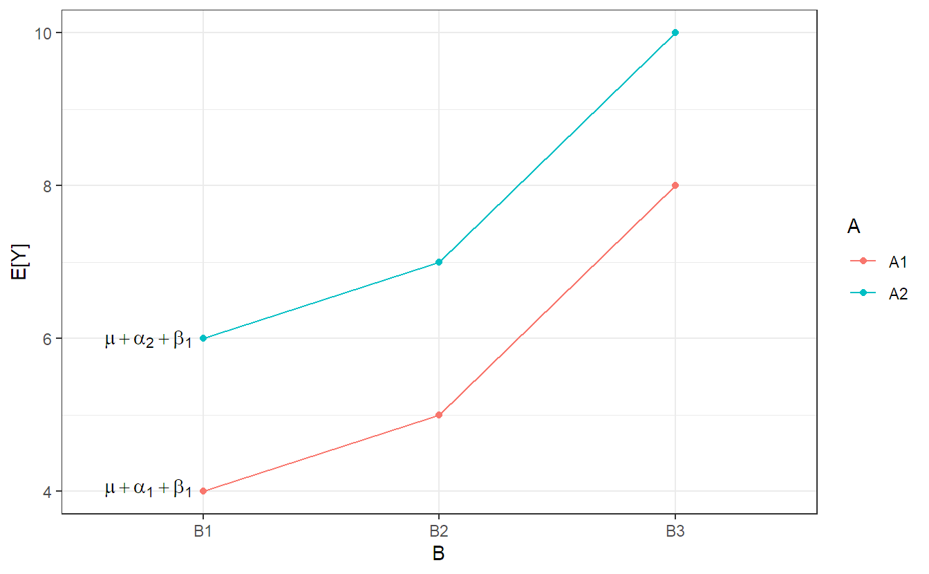
A model without interaction term is additive. This means that the effect of \(A\) does not depend on the level of \(B\), and vice versa, “it is always the same, no matter what the level of the other factor”. An illustration (for a general setup) can be found in Figure 4.3, where we see that the lines are parallel. This means that changing \(A\) from level 1 to level 2 has always the same effect (here, an increase by 2 units). Similarly, the effect of changing \(B\) does not depend on the level of \(A\) (here, an increase by 1 and 3 units if we change \(B\) from level 1 to 2, and 2 to 3, respectively).
Typically, we use sum-to-zero side constraints, i.e., \(\sum_{i=1}^a \alpha_i = 0\) and \(\sum_{j=1}^b \beta_j = 0\) for the main effects. Hence, the main effects have \(a - 1\) and \(b - 1\) degrees of freedom, respectively, “as before”. For the interaction effect we have to make sure that it contains nothing which is row- or column-specific, that is why we have the side constraints \(\sum_{i=1}^a (\alpha \beta)_{ij} = 0\) (sum across rows) for all \(j\)’s and \(\sum_{j=1}^b (\alpha \beta)_{ij} = 0\) (sum across columns) for all \(i\)’s. Therefore, the degrees of freedom of the interaction term are \((a - 1)(b - 1)\). Rule to remember: The degrees of freedom of the interaction effect are the product of the degrees of freedom of the involved main effects.
4.2.1 Parameter Estimation
As usual, we estimate parameters using the principles of least squares. Using sum-to-zero side constraints, one can show that we get the parameter estimates listed in Table 4.4. As before, if we replace an index with a dot, we take the mean, or the sum, over that dimension. For example, \(\overline{y}_{1\cdot\cdot}\) is the mean over all observations in the first row: \(y_{1jk}\), \(j = 1, \ldots, b\) and \(k = 1, \ldots, n\). To calculate \(\widehat{\alpha}_1\), we simply determine the deviation of the mean of the first row \(\overline{y}_{1\cdot\cdot}\) from the overall mean \(\overline{y}_{\cdot\cdot\cdot}\), i.e., \[ \widehat{\alpha}_1 = \overline{y}_{1\cdot\cdot} - \overline{y}_{\cdot\cdot\cdot}. \]
| Parameter | Estimate |
|---|---|
| \(\mu\) | \(\widehat{\mu} = \overline{y}_{\cdot\cdot\cdot}\) |
| \(\alpha_i\) | \(\widehat{\alpha}_i = \overline{y}_{i\cdot\cdot} - \overline{y}_{\cdot\cdot\cdot}\) |
| \(\beta_j\) | \(\widehat{\beta}_j = \overline{y}_{\cdot j \cdot} - \overline{y}_{\cdot\cdot\cdot}\) |
| \((\alpha \beta)_{ij}\) | \(\widehat{(\alpha \beta)}_{ij} = \overline{y}_{ij\cdot} - \widehat{\mu} - \widehat{\alpha}_i - \widehat{\beta}_j\) |
Combining all this information, we estimate the expected value of the response \(Y_{ijk}\) for \(A\) at level \(i\) and \(B\) at level \(j\) as \[ \widehat{\mu} + \widehat{\alpha}_i + \widehat{\beta}_j + \widehat{(\alpha \beta)}_{ij} = \overline{y}_{i j \cdot} \] which is nothing more than the mean of the observations in the corresponding cell (which is hopefully no surprise). However, note that we untangled the effect with respect to the two main effects and the interaction. If we would use an unstructured cell means model with \(a\cdot b\) different cell means, we would get the very same estimates for the cell means.
If we carefully inspect the parameter estimates in Table 4.4, we observe that for the main effects, we use an estimate that completely ignores the other factor. We basically treat the problem as a one-way ANOVA model. This is a consequence of the balanced design. For all levels of \(A\) we have the “same population” of levels of \(B\). Hence, if we compare \(\overline{y}_{1\cdot\cdot}\) (average over the first row) with \(\overline{y}_{2\cdot\cdot}\) (average over second row), the effect is only due to changing \(A\) from level 1 to level 2. In regression terminology, we would call this an orthogonal design.
In R, we fit the model using the function aov. For our example, the model of Equation 4.1 would be written as dist ~ brand + underground + brand:underground in R formula notation. The colon “:” indicates an interaction effect. Separate terms are connected by a “+”. Alternatively, the asterisk “*” is a useful shorthand notation to include two main effects as well as their interaction, i.e., the same model could also be specified as dist ~ brand * underground. A model which contains only the main effects of brand and underground (without interaction effect) would be specified as dist ~ brand + underground.
options(contrasts = c("contr.sum", "contr.poly"))
fit.bike <- aov(dist ~ brand * underground, data = bike)
coef(fit.bike)
## (Intercept) brand1 underground1
## 886.28 26.61 189.39
## underground2 brand1:underground1 brand1:underground2
## -29.94 -63.61 19.06The remaining coefficients can be obtained by making use of the sum-to-zero constraint. An easier way is to use the function dummy.coef
dummy.coef(fit.bike)## Full coefficients are
##
## (Intercept): 886.3
## brand: 1 2
## 26.61 -26.61
## underground: soft rocky extreme
## 189.39 -29.94 -159.44
## brand:underground: 1:soft 2:soft 1:rocky 2:rocky 1:extreme 2:extreme
## -63.61 63.61 19.06 -19.06 44.56 -44.56For example, the cell mean of combination brand 1 and underground soft can be explained as the sum of (Intercept): \(\widehat{\mu} = 886.28\), main effect of brand 1: \(\widehat{\alpha}_1 = 26.61\), main effect of underground soft: \(\widehat{\beta}_1 = 189.39\) and interaction effect of the combination of the two levels of brand and underground 1:soft: \(\widehat{(\alpha\beta)}_{11} = -63.61\).
As an exercise and for a better understanding of the parameter estimates, you can of course also manually calculate, or verify, the parameter estimates using the information in Table 4.5.
| Brand | Soft | Rocky | Extreme | $\overline{y}_{i\cdot\cdot}$ |
|---|---|---|---|---|
| 1 | 1014, 1062, 1040 | 884, 929, 893 | 824, 778, 792 | $\overline{y}_{1\cdot\cdot} = 912.89$ |
| 2 | 1095, 1116, 1127 | 818, 794, 820 | 642, 633, 692 | $\overline{y}_{2\cdot\cdot} = 859.67$ |
| $\overline{y}_{\cdot j\cdot}$ | $\overline{y}_{\cdot1\cdot} = 1075.67$ | $\overline{y}_{\cdot2\cdot} = 856.33$ | $\overline{y}_{\cdot3\cdot} = 726.83$ | $\overline{y}_{\cdot\cdot\cdot} = 886.28$ |
4.2.2 Tests
As in the case of the one-way ANOVA, the total sum of squares \(SS_T\) can be (uniquely) partitioned into different sources, i.e., \[ SS_T = SS_A + SS_B + SS_{AB} + SS_E, \] where the individual terms are given in Table 4.6.
| Source | Sum of Squares |
|---|---|
| \(A\) (“between rows”) | \(SS_A = \sum_{i=1}^a b n (\widehat{\alpha}_i)^2\) |
| \(B\) (“between columns”) | \(SS_B = \sum_{j=1}^b a n (\widehat{\beta}_j)^2\) |
| \(AB\) (“correction”) | \(SS_{AB} = \sum_{i=1}^a \sum_{j=1}^b n (\widehat{\alpha\beta})_{ij}^2\) |
| \(\text{Error}\) (“within cells”) | \(SS_E = \sum_{i=1}^a \sum_{j=1}^b \sum_{k=1}^n (y_{ijk} - \overline{y}_{ij\cdot})^2\) |
| \(\textrm{Total}\) | \(SS_T = \sum_{i=1}^a \sum_{j=1}^b \sum_{k=1}^n (y_{ijk} - \overline{y}_{\cdot\cdot\cdot})^2\) |
By calculating the corresponding mean squares, we can construct an ANOVA table, see Table 4.7.
| Source | df | SS | Mean Squares | \(F\)-ratio |
|---|---|---|---|---|
| \(A\) | \(a - 1\) | \(SS_A\) | \(MS_A = \frac{SS_A}{a-1}\) | \(\frac{MS_A}{MS_E}\) |
| \(B\) | \(b - 1\) | \(SS_B\) | \(MS_B = \frac{SS_B}{b-1}\) | \(\frac{MS_B}{MS_E}\) |
| \(AB\) | \((a-1)(b-1)\) | \(SS_{AB}\) | \(MS_{AB} = \frac{SS_{AB}}{(a-1)(b-1)}\) | \(\frac{MS_{AB}}{MS_E}\) |
| \(\textrm{Error}\) | \(ab(n-1)\) | \(SS_E\) | \(MS_E = \frac{SS_E}{ab(n-1)}\) |
Note: The degrees of freedom of the error term is nothing more than the degrees of freedom of the total sum of squares (\(abn - 1\), number of observations minus 1) minus the sum of the degrees of freedom of all other effects.
As in the one-way ANOVA situation, we can construct global tests for the main effects and the interaction effect:
Interaction effect: The null hypothesis that there is no interaction effect can be translated as: “The effect of factor \(A\) does not depend on the level of factor \(B\) (or the other way round). Or, the main effects model is enough.” In the example it would mean: “The effect of underground does not depend on brand.” The model could be visualized as in Figure 4.3, i.e., with parallel lines. In formulas we have \[\begin{align*} H_0&: (\alpha \beta)_{ij} = 0 \textrm{ for all } i,j \\ H_A&: \textrm{at least one } (\alpha \beta)_{ij} \neq 0 \end{align*}\] Under \(H_0\) it holds that \(\frac{MS_{AB}}{MS_E} \sim F_{(a-1)(b-1), \, ab(n-1)}\).
Main effect of A: The null hypothesis that there is no main effect of \(A\) can be translated as: “The (average) effect of factor \(A\) does not exist.” In the example it would mean: “There is no effect of brand when averaged over all levels of underground. Or, both brands have the same expected distance when averaged over all levels of underground.” In formulas we have \[\begin{align*} H_0&: \alpha_i = 0 \textrm{ for all } i \\ H_A&: \textrm{at least one } \alpha_i \neq 0 \end{align*}\] Under \(H_0\) it holds that \(\frac{MS_A}{MS_E} \sim F_{a-1, \, ab(n-1)}\).
Main effect of B: The null hypothesis that there is no main effect of \(B\) can be translated as: “The (average) effect of factor \(B\) does not exist.” In the example it would mean: “There is no effect of underground when averaged over both brands. Or, all undergrounds have the same expected distance when averaged over both brands.” In formulas we have \[\begin{align*} H_0&: \beta_j = 0 \textrm{ for all } j \\ H_A&: \textrm{at least one } \beta_j \neq 0 \end{align*}\] Under \(H_0\) it holds that \(\frac{MS_B}{MS_E} \sim F_{b-1, \, ab(n-1)}\).
The \(F\)-distributions all follow the same pattern: The degrees of freedom are given by the numerator and the denominator of the corresponding \(F\)-ratio, respectively.
In R, we get the ANOVA table and the corresponding p-values again with the summary function. We read the following R output from bottom to top. This means that we first check whether we need the interaction term or not. If there is no evidence of interaction, we continue with the inspection of the main effects.
summary(fit.bike)## Df Sum Sq Mean Sq F value Pr(>F)
## brand 1 12747 12747 24.0 0.00037
## underground 2 373124 186562 351.5 2.2e-11
## brand:underground 2 38368 19184 36.1 8.3e-06
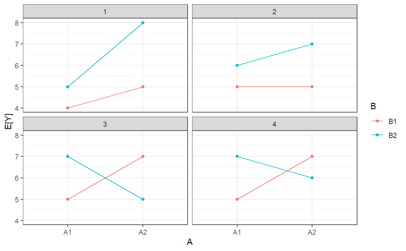
## Residuals 12 6369 531There is evidence of an interaction between brand and underground as the p-value is very small (line brand:underground). This finding is consistent with what we have observed in the interaction plot in Figure 4.1. This means that there is statistical evidence that the effect of underground depends on brand. Typically, the effect of underground is then analyzed for each level of brand separately. From the interaction plot we can observe that this interaction is mainly caused by the different behavior for underground soft. In the presence of a significant interaction, the main effects (which are average effects) are typically not very interesting anymore. For example, if we have a data set where the interaction is significant but one of the main effects is not, we should not conclude that there is no effect of the corresponding factor. The effect simply depends on the level of the other factor. Some of the possible situations for the true parameter values of [Equation Equation 4.1} for the situation of two factors with two levels each are illustrated in Figure 4.4. In panel 1, the strength of the effect of \(A\) depends on the level of \(B\), but the sign is always the same (both the main effects of \(A\) and \(B\) and the interaction are nonzero). In panel 2, there is no effect of \(A\) for \(B\) at level 1, but at level 2 (again, both the main effects of \(A\) and \(B\) and the interaction are nonzero). In panel 3 we have the very special situation that both main effects vanish, but the interaction is very pronounced. In panel 4, the sign of the effect of \(A\) depends on the level of \(B\) (both the main effects of \(A\) and \(B\) and the interaction are nonzero).
In our example, we could start analyzing the effect of brand for each level of underground by inspecting some specific questions using appropriate contrasts (this is of course also meaningful if such a question was planned beforehand). For example, what is the difference between the two brands for underground soft? From a technical point of view, one way of doing this is by constructing what we would call a hyper-factor which has as levels all possible combinations of brand and underground; this is equivalent to the full model but typically easier to handle with respect to the mentioned contrast. In R, we can easily do this with the function interaction which “glues together” the information from two factors.
bike[,"trt.comb"] <- interaction(bike[, "brand"],
                                 bike[, "underground"])
levels(bike[,"trt.comb"])
## [1] "1.soft" "2.soft" "1.rocky" "2.rocky" "1.extreme" "2.extreme"We use this hyper-factor to fit a one-way ANOVA model. Again, this gives the same estimated cell means as the two-way ANOVA model, but it is easier for handling the contrast later on.
fit.bike.comb <- aov(dist ~ trt.comb, data = bike)Now we answer the previous question with an appropriate contrast (here, using package multcomp).
library(multcomp)
## Brand 1 vs. brand 2 for underground soft
fit.glht <- glht(fit.bike.comb,
                 linfct = mcp(trt.comb = c(1, -1, 0, 0, 0, 0)))
confint(fit.glht)
## ...
## Linear Hypotheses:
## Estimate lwr upr
## 1 == 0 -74.000 -114.983 -33.017This means that for underground soft, a 95% confidence interval for the difference between brand 1 and brand 2 is given by \([-114.98, -33.02]\).
Note: Both multcomp and emmeans can be used to directly handle contrasts using the two-way ANOVA model (with interaction). However, interpretation can be difficult (typically you would also see a corresponding warning message). This is why we prefer to explicitly fit the corresponding cell means model and apply the contrast there.
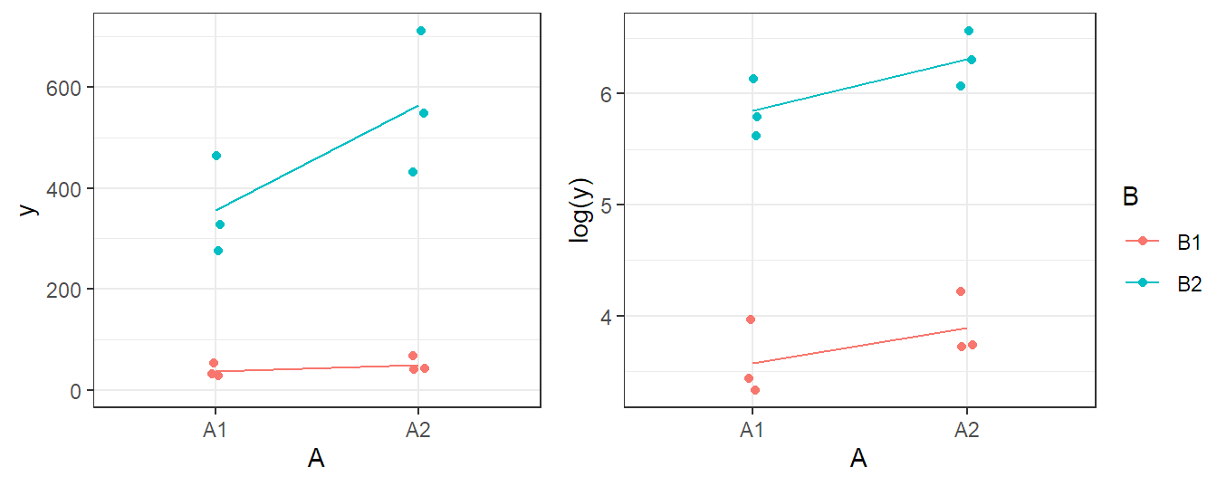
Whether an interaction is needed or not might also depend on the scale on which we are analyzing the response. A famous example is the logarithm. Effects that are multiplicative on the original scale become additive on the log-scale, i.e., no interaction is needed on the log-scale. For example, see Figure 4.5. In the left panel, we can observe that there might be an interaction effect and that variation is larger for large values of the response. In the right panel, we see the corresponding interaction plot when taking the logarithm of the response. The interaction effect seems to have gone and in addition, variability is much more constant than before. This phenomenon is very common in practice.
4.2.3 Single Observations per Cell
If we only have a single observation in each “cell” (\(n = 1\)), we cannot do statistical inference anymore with a model including the interaction. The reason is that we have no idea of the experimental error (the variation between experimental units getting the same treatment). From a technical point of view, fitting a model with an interaction term would lead to a perfect fit with all residuals being exactly zero.
However, we can still fit a main effects only model. If the data generating mechanism actually contains an interaction, we are fitting a wrong model. The consequence is that the estimate of the error variance will be biased (upward). Hence, the corresponding tests will be too conservative, meaning p-values will be too large and confidence intervals too wide. This is not a problem as the type I error rate is still controlled; we “just” lose power.
An alternative approach would be to use a Tukey one-degree of freedom interaction (Tukey 1949), a highly structured form of interaction effect where the interaction effect actually is assumed to be proportional to the product of the corresponding main effects. This would only use one additional parameter for the interaction term.
4.2.4 Checking Model Assumptions
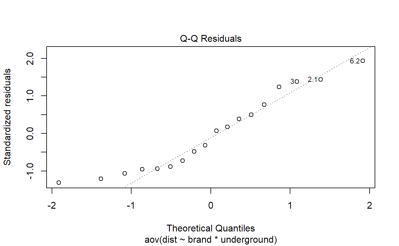
As in Section 2.2, we use the QQ-plot and the Tukey-Anscombe plot to check the model assumptions. Let us use the two-way ANOVA model of the mountain bike tire data set stored in object fit.bike as an example. We start with the QQ-plot of the residuals:
plot(fit.bike, which = 2)If in doubt that the QQ-plot in Figure 4.6 is still OK, we could use the function qqPlot of the package car as discussed in Section 2.2.1. Alternatively, we can always compare it to a couple of “nice” simulated QQ-plots of the same sample size using the following command (give it a try, output not shown).
Our QQ-plot in Figure 4.6 looks like one from simulated data. Hence, there is no evidence of a violation of the normality assumption of the error term.
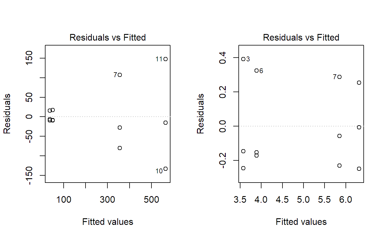
The Tukey-Anscombe plot looks OK too in the sense that there is no evidence of non-constant variance:
plot(fit.bike, which = 1, add.smooth = FALSE)To illustrate, the Tukey-Anscombe plots for two-way ANOVA models (including interaction) using the data of Figure 4.5 are shown in Figure 4.7. On the original scale, a funnel-like shape is clearly visible. This is a sign that transforming the response with the logarithm will stabilize the variance, as can be observed from the plot on the transformed data.
4.2.5 Unbalanced Data
Introduction
We started with the very strong assumption that our data is balanced, i.e., for every treatment “setting,” e.g., a specific combination of underground and brand, we have the same number of replicates. This assumption made our life “easy” in the sense that we could uniquely decompose total variability into different sources and we could estimate the parameters of the coefficients of a factor by ignoring the other factors. In practice, data is typically not balanced. Think for example of a situation where something goes wrong with an experiment in some of the settings. With such unbalanced data or unbalanced design, the aforementioned properties typically do not hold anymore. We still use least squares to estimate the parameters. The estimates will look more complicated. However, this is not a problem these days as we can easily calculate them using R. More of a problem is the fact that the sum of squares cannot be uniquely partitioned into different sources anymore. This means that for some part of the variation of the data, it is not clear what source we should attribute it to.
Typically, people use an appropriate model comparison approach instead. As seen before, for example in Table 4.6, the sum of squares of a factor can be interpreted as the reduction of residual sum of squares when adding the corresponding factor to the model. In the balanced situation, it would not matter whether the remaining factors are in the model or not; the reduction is always the same. Unfortunately, for unbalanced data this property does not hold anymore.
We follow Oehlert (2000) and use the following notation: With SS(B | 1, A) we denote the reduction in residual sum of squares when comparing the model (1, A, B) (= y ~ A + B) with (1, A) (= y ~ A). The 1 is the overall mean \(\mu\) (that does not appear explicitly in the R model formula). Interpretation of the corresponding test is as follows: “Do we need factor B in the model if we already have factor A, or after having controlled for factor A?”. There are different “ways” or “types” of model comparison approaches:
- Type I (sequential): Sequentially build up model (depends on the ordering of the model terms!)
SS(A | 1)SS(B | 1, A)SS(AB | 1, A, B)
- Type II (hierarchical): Controlling for the influence of the largest hierarchical model not including the term of interest. With hierarchical we mean that whenever an interaction is included in the model, the corresponding main effects are included too.
SS(A | 1, B)SS(B | 1, A)SS(AB | 1, A, B)
- Type III (fully adjusted): Controlling for all other terms.
SS(A | 1, B, AB)SS(B | 1, A, AB)SS(AB | 1, A, B)
Type I is what you get with summary of an aov object (like summary(fit.bike)) or if you call the function anova using a single argument, e.g., anova(fit.bike). Hence, for unbalanced data you get different results whether you write y ~ A * B or y ~ B * A, see also R FAQ 7.18. For type II we can either use the function Anova in the package car or we could compare the appropriate models with the function anova ourselves. For type III we can use the command drop1; we have to be careful that we set the contrast option to contr.sum in this special situation for technical reasons, see also the warning in the help file of the function Anova of package car.
Typically, we take \(MS_E\) from the full model (including all terms) as the estimate for the error variance to construct the corresponding \(F\)-tests.
Note that interpretation of the test depends on the type that we use. This can be seen from the following remarks.
Some Technical Remarks
We use the notation \[ Y_{ijk} = \mu_{ij} + \epsilon_{ijk} \] where \(\mu_{ij} = \mu + \alpha_i + \beta_j + (\alpha \beta)_{ij}\). This means we use a cell means model with expected values \(\mu_{ij}\). We denote the corresponding sample sizes for the level combination \((i, j)\) with \(n_{ij} > 0\). It can be shown (Speed, Hocking, and Hackney 1978) that both type I and type II sum of squares lead to tests that involve null hypotheses that depend on the sample sizes of the individual cells!
More precisely, for example for the main effect \(A\) we have:
For type I sum of squares, we implicitly test the null hypothesis \[ H_0: \sum_{j = 1}^b \frac{n_{1j}}{n_{1\cdot}} \mu_{1j} = \cdots = \sum_{j = 1}^b \frac{n_{aj}}{n_{a\cdot}} \mu_{aj} \] where \(n_{i\cdot}\) is the sum of the corresponding \(n_{ij}\)’s. The above equation simply means that across all rows, a weighted mean of the \(\mu_{ij}\)’s is the same. Note that the weights depend on the observed sample sizes \(n_{ij}\). Therefore, the observed sample sizes dictate our null hypothesis! Interpretation of such a research question is rather difficult.
Similarly, for type II sum of squares we get a more complicated formula involving \(n_{ij}\)’s.
For type III sum of squares we have \[ H_0: \overline{\mu}_{1\cdot} = \cdots = \overline{\mu}_{a\cdot} \] where \(\overline{\mu}_{i\cdot} = \frac{1}{b} \sum_{l = 1}^b \mu_{il}\) which is the unweighted mean of the corresponding \(\mu_{ij}\)’s. This can be reformulated as \[ H_0: \alpha_1 = \cdots = \alpha_a \] This is what we have used so far, and more importantly, does not depend on \(n_{ij}\).
We can also observe that for a balanced design, we test the same null hypothesis, no matter what type we use.
Unbalanced Data Example
We have a look at some simulated data about a sports experiment using a factorial design with the factor “training method” (method, with levels conventional and new) and the factor “energy drink” (drink, with levels A and B). The response is running time in seconds for a specific track.
book.url <- "https://stat.ethz.ch/~meier/teaching/book-anova"
running <- read.table(file.path(book.url, "data/running.dat"),
                      header = TRUE)
str(running)
## 'data.frame': 70 obs. of 3 variables:
## $ method: chr "new" "new" ...
## $ drink : chr "A" "A" ...
## $ y : num 40.6 49.7 42.1 42.2 39 44.2 ...The output of xtabs gives us all the \(n_{ij}\)’s.
xtabs(~ method + drink, data = running)## drink
## method A B
## conventional 10 40
## new 10 10Clearly, this is an unbalanced data set. We use contr.sum; otherwise, type III sum of squares will be wrong (technical issue).
options(contrasts = c("contr.sum", "contr.poly"))
## Type I sum of squares
fit <- aov(y ~ method * drink, data = running)
summary(fit)
## Df Sum Sq Mean Sq F value Pr(>F)
## method 1 2024 2024 263.72 < 2e-16
## drink 1 455 455 59.32 9.1e-11
## method:drink 1 29 29 3.79 0.056
## Residuals 66 507 8For example, the row method tests the null hypothesis \[
H_0: 0.2 \cdot \mu_{11} + 0.8 \cdot \mu_{12} = 0.5 \cdot \mu_{21} +
0.5 \cdot \mu_{22}
\] (because 80% of training method conventional use energy drink B).
Now we change the order of the factors in the model formula.
##              Df Sum Sq Mean Sq F value Pr(>F)
## drink         1   1146    1146  149.30 <2e-16
## method        1   1333    1333  173.74 <2e-16
## drink:method  1     29      29    3.79  0.056
## Residuals    66    507       8
We can see that the sum of squares depend on the ordering of the model terms in the model formula if we use a type I approach (if method comes first, we get 2024, otherwise 1333). Hence, we also get different \(F\)-ratios and different p-values. However, the p-values of the main effects are very small here, no matter what order we use.
We can easily get type II sum of squares with the package car.
## Anova Table (Type II tests)
##
## Response: y
##              Sum Sq Df F value  Pr(>F)
## method         1333  1  173.74 < 2e-16
## drink           455  1   59.32 9.1e-11
## method:drink     29  1    3.79   0.056
## Residuals       507 66
We could also use the Anova function for type III sum of squares, but drop1 will do the job too.
## Type III sum of squares
drop1(fit, scope = ~., test = "F", data = running)
## or: Anova(fit, type = "III", data = running)
## Single term deletions
##
## Model:
## y ~ method * drink
## Df Sum of Sq RSS AIC F value Pr(>F)
## <none> 507 146
## method 1 1352 1859 236 176.21 < 2e-16
## drink 1 484 991 192 63.09 3.3e-11
## method:drink 1 29 536 148 3.79 0.056Now the row method tests the null hypothesis \[
H_0: \frac{1}{2} \cdot \mu_{11} + \frac{1}{2} \cdot \mu_{12} =
\frac{1}{2} \cdot \mu_{21} + \frac{1}{2} \cdot \mu_{22},
\] which is nothing but saying that the (unweighted) “row-average” of the \(\mu_{ij}\)’s is constant. Here, the actual sample sizes do not play a role anymore. Note that we always get the same result for the interaction effect, no matter what type we use.
4.3 Outlook
4.3.1 More Than Two Factors
We can easily extend the model to more than two factors. If we have three factors \(A\), \(B\) and \(C\) (with \(a\), \(b\) and \(c\) levels, respectively), we have \(3\) main effects, \(3 \cdot 2 / 2 = 3\) two-way interactions (the “usual” interaction so far) and one so-called three-way interaction. We omit the mathematical model formulation and work directly with the corresponding R code. In R, we would write y ~ A * B * C for a three-way ANOVA model including all main effects, all two-way interactions and a three-way interaction. An equivalent formulation would be y ~ A + B + C + A:B + A:C + B:C + A:B:C.
Main effects are interpreted as average effects, two-way interaction effects are interpreted as deviations from the main effects model, i.e., the correction for an effect that depends on the level of the other factor, and the three-way interaction is an adjustment of the two-way interaction depending on the third factor. Or in other words, if there is a three-way interaction it means that the effect of factor \(A\) depends on the level combination of the factors \(B\) and \(C\), i.e., each level combination of \(B\) and \(C\) has its own effect of \(A\). This typically makes interpretation difficult.
In a balanced design, the model parameters are estimated as “usual.” To estimate the three-way interaction, we simply subtract all estimates of the main effects and the two-way interactions. The degrees of freedom for the three-way interaction are the product of the degrees of freedom of all involved factors.
A potential ANOVA table for a balanced design with \(n\) replicates in each cell is given in Table 4.8.
| Source | df | \(F\)-ratio | |
|---|---|---|---|
| \(A\) | \(a - 1\) | \(\frac{MS_A}{MS_E}\) | |
| \(B\) | \(b - 1\) | \(\frac{MS_B}{MS_E}\) | |
| \(C\) | \(c - 1\) | \(\frac{MS_C}{MS_E}\) | |
| \(AB\) | \((a-1)(b-1)\) | \(\frac{MS_{AB}}{MS_E}\) | |
| \(AC\) | \((a-1)(c-1)\) | \(\frac{MS_{AC}}{MS_E}\) | |
| \(BC\) | \((b-1)(c-1)\) | \(\frac{MS_{BC}}{MS_E}\) | |
| \(ABC\) | \((a-1)(b-1)(c-1)\) | \(\frac{MS_{ABC}}{MS_E}\) | |
| \(\textrm{Error}\) | \(abc(n-1)\) |
The model with a three-way interaction is flexible enough to model \(abc\) different cell means! We also observe that the three-way interaction typically has large degrees of freedom (meaning, it needs a lot of parameters!). We can only do statistical inference about the three-way interaction if we have multiple observations in the individual cells. If we would only have one observation in each cell (\(n = 1\)), we could still fit the model y ~ A + B + C + A:B + A:C + B:C. This means that we drop the highest-order interaction and “pool it” into the error term. This is quite a common strategy, especially if we have more than three factors. Most often, the effect size of the most complex interaction is assumed to be small or zero. Hence, the corresponding term can be dropped from the model to save degrees of freedom. Ideally, these decisions are made before looking at the data. Otherwise, dropping all the insignificant terms from the model and putting them into the error term will typically lead to biased results (see also the comments in section 8.9 in Oehlert 2000). This will make the remaining model terms look too significant, i.e., we declare too many effects as significant although they are actually not. This means that the type I error rate is not being controlled anymore. In addition, the corresponding confidence intervals will be too narrow.
A common question is: “Can I test a certain interaction with my data?”. If multiple observations are available for each combination of the levels of the involved factors, we can test the interaction. We do not have to consider the remaining factors in the model. For example, if we have three factors \(A\), \(B\) and \(C\), we can do statistical inference about the interaction between \(A\) and \(B\) if we have multiple observations for each combination of the levels of \(A\) and \(B\), even if they correspond to different levels of \(C\). Hence, as already mentioned, even if we have only one observation for each treatment combination of \(A\), \(B\) and \(C\) we can do statistical inference about two-way interaction effects (but not about the three-way interaction).
4.3.2 Nonparametric Alternatives
Unfortunately, nonparametric approaches are not very common for factorial designs. For example, when using randomization tests, it is much more difficult to isolate the effect of interest (say, a certain main effect). More information can be found for example in Edgington and Onghena (2007) or Anderson (2001).
